

156
9 Study of Optical Properties of Biotissues by the Intracavity …
E
−
n (ξ
1 ) = C n H n
ξ
1 ·
√
2
ω
exp
i(n + 1/2)g − ik L −
iξ
2
1
q −
.
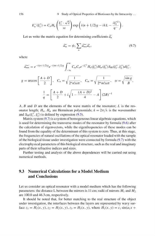
Let us write the matrix equation for determining coefficients
a n
a m = ψ 1
n
a mn
a n ,
(9.7)
where
a mn = e
−i(n+1/2)g e
−i(m+1/2)g
∞
−∞
C m C n e
−ξ
2
1 H n (ξ
1 )H m (ξ
1 )S 00 (ξ
1 , ξ
2 )dξ
1 ,
g = arccos
A + D
2
, C n =
1
2 n n!ωπ
, C m =
1
2 m m!ωπ
, ω =
sin g
B
,
1
q
=
A + D
2
+ i
1 −
(A + D) 2
4
− A
(2B)
−1
A, B and D are the elements of the wave matrix of the resonator; L is the resonator length; H n , H m are Hermitean polynomials; k = 2π/λ is the wavenumber
and S 00 (ξ
1 , ξ
2 ) is defined by expression (9.5).
Matrix system (9.7) is a system of homogeneous linear algebraic equations, which
is used for determining the transverse modes of the resonator by formula (9.6) after
the calculation of eigenvectors, while the eigenfrequencies of these modes can be
found from the equality of the determinant of this system to zero. Thus, at this stage,
the frequencies of natural oscillations of the optical resonator loaded with the sample
of the biological tissue under investigation were connected by formula (9.7) with the
electrophysical parameters of this biological structure, such as the real and imaginary
parts of their refractive indices and sizes.
Further testing and analysis of the above dependences will be carried out using
numerical methods.
9.3 Numerical Calculations for a Model Medium
and Conclusions
Let us consider an optical resonator with a model medium which has the following
parameters: the distance L between the mirrors is 11 cm; radii of mirrors M 1 and M 2
are 100.0 and 46.3 cm, respectively.
It should be noted that, for better matching to the real structure of the object
under investigation, the interfaces between the layers are represented by wavy surface z 1 = H 1 (x, y), z 2 = H 2 (x, y), z 3 = H 3 (x, y), where H 1 (x, y) = c 1 sin(a 1 x +
9 Study of Optical Properties of Biotissues by the Intracavity …
E
−
n (ξ
1 ) = C n H n
ξ
1 ·
√
2
ω
exp
i(n + 1/2)g − ik L −
iξ
2
1
q −
.
Let us write the matrix equation for determining coefficients
a n
a m = ψ 1
n
a mn
a n ,
(9.7)
where
a mn = e
−i(n+1/2)g e
−i(m+1/2)g
∞
−∞
C m C n e
−ξ
2
1 H n (ξ
1 )H m (ξ
1 )S 00 (ξ
1 , ξ
2 )dξ
1 ,
g = arccos
A + D
2
, C n =
1
2 n n!ωπ
, C m =
1
2 m m!ωπ
, ω =
sin g
B
,
1
q
=
A + D
2
+ i
1 −
(A + D) 2
4
− A
(2B)
−1
A, B and D are the elements of the wave matrix of the resonator; L is the resonator length; H n , H m are Hermitean polynomials; k = 2π/λ is the wavenumber
and S 00 (ξ
1 , ξ
2 ) is defined by expression (9.5).
Matrix system (9.7) is a system of homogeneous linear algebraic equations, which
is used for determining the transverse modes of the resonator by formula (9.6) after
the calculation of eigenvectors, while the eigenfrequencies of these modes can be
found from the equality of the determinant of this system to zero. Thus, at this stage,
the frequencies of natural oscillations of the optical resonator loaded with the sample
of the biological tissue under investigation were connected by formula (9.7) with the
electrophysical parameters of this biological structure, such as the real and imaginary
parts of their refractive indices and sizes.
Further testing and analysis of the above dependences will be carried out using
numerical methods.
9.3 Numerical Calculations for a Model Medium
and Conclusions
Let us consider an optical resonator with a model medium which has the following
parameters: the distance L between the mirrors is 11 cm; radii of mirrors M 1 and M 2
are 100.0 and 46.3 cm, respectively.
It should be noted that, for better matching to the real structure of the object
under investigation, the interfaces between the layers are represented by wavy surface z 1 = H 1 (x, y), z 2 = H 2 (x, y), z 3 = H 3 (x, y), where H 1 (x, y) = c 1 sin(a 1 x +