

4 The Analysis of Event-Related Potentials
67
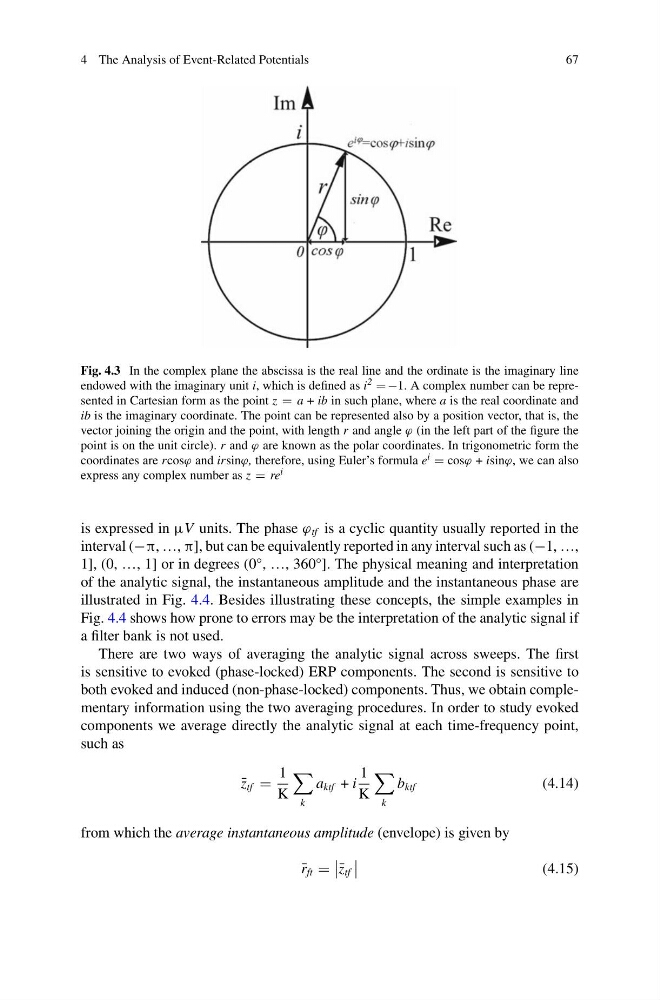
Fig. 4.3 In the complex plane the abscissa is the real line and the ordinate is the imaginary line
endowed with the imaginary unit i, which is defined as i 2 −1. A complex number can be represented in Cartesian form as the point z a + ib in such plane, where a is the real coordinate and
ib is the imaginary coordinate. The point can be represented also by a position vector, that is, the
vector joining the origin and the point, with length r and angle ϕ (in the left part of the figure the
point is on the unit circle). r and ϕ are known as the polar coordinates. In trigonometric form the
coordinates are rcosϕ and irsinϕ, therefore, using Euler’s formula e i cosϕ + isinϕ, we can also
express any complex number as z re i
is expressed in μV units. The phase ϕ tf is a cyclic quantity usually reported in the
interval (−π, …, π], but can be equivalently reported in any interval such as (−1, …,
1], (0, …, 1] or in degrees (0°, …, 360°]. The physical meaning and interpretation
of the analytic signal, the instantaneous amplitude and the instantaneous phase are
illustrated in Fig. 4.4. Besides illustrating these concepts, the simple examples in
Fig. 4.4 shows how prone to errors may be the interpretation of the analytic signal if
a filter bank is not used.
There are two ways of averaging the analytic signal across sweeps. The first
is sensitive to evoked (phase-locked) ERP components. The second is sensitive to
both evoked and induced (non-phase-locked) components. Thus, we obtain complementary information using the two averaging procedures. In order to study evoked
components we average directly the analytic signal at each time-frequency point,
such as
¯
z tf
1
K
k
a ktf + i
1
K
k
b ktf
(4.14)
from which the average instantaneous amplitude (envelope) is given by
¯
r ft
¯
z tf
(4.15)
67
Fig. 4.3 In the complex plane the abscissa is the real line and the ordinate is the imaginary line
endowed with the imaginary unit i, which is defined as i 2 −1. A complex number can be represented in Cartesian form as the point z a + ib in such plane, where a is the real coordinate and
ib is the imaginary coordinate. The point can be represented also by a position vector, that is, the
vector joining the origin and the point, with length r and angle ϕ (in the left part of the figure the
point is on the unit circle). r and ϕ are known as the polar coordinates. In trigonometric form the
coordinates are rcosϕ and irsinϕ, therefore, using Euler’s formula e i cosϕ + isinϕ, we can also
express any complex number as z re i
is expressed in μV units. The phase ϕ tf is a cyclic quantity usually reported in the
interval (−π, …, π], but can be equivalently reported in any interval such as (−1, …,
1], (0, …, 1] or in degrees (0°, …, 360°]. The physical meaning and interpretation
of the analytic signal, the instantaneous amplitude and the instantaneous phase are
illustrated in Fig. 4.4. Besides illustrating these concepts, the simple examples in
Fig. 4.4 shows how prone to errors may be the interpretation of the analytic signal if
a filter bank is not used.
There are two ways of averaging the analytic signal across sweeps. The first
is sensitive to evoked (phase-locked) ERP components. The second is sensitive to
both evoked and induced (non-phase-locked) components. Thus, we obtain complementary information using the two averaging procedures. In order to study evoked
components we average directly the analytic signal at each time-frequency point,
such as
¯
z tf
1
K
k
a ktf + i
1
K
k
b ktf
(4.14)
from which the average instantaneous amplitude (envelope) is given by
¯
r ft
¯
z tf
(4.15)