

66
M. Congedo
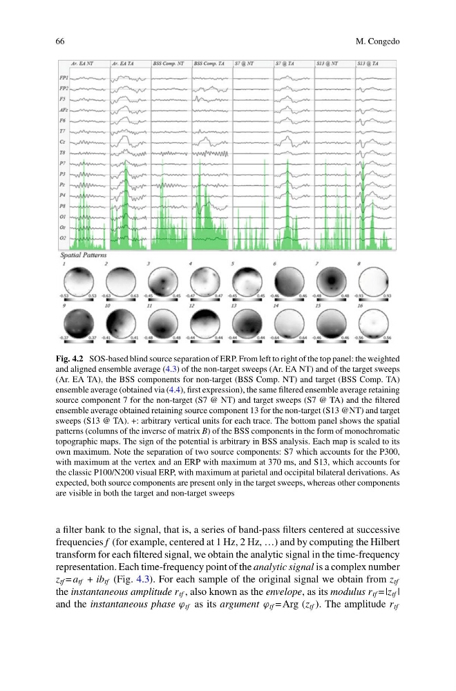
Fig. 4.2 SOS-based blind source separation of ERP. From left to right of the top panel: the weighted
and aligned ensemble average (4.3) of the non-target sweeps (Ar. EA NT) and of the target sweeps
(Ar. EA TA), the BSS components for non-target (BSS Comp. NT) and target (BSS Comp. TA)
ensemble average (obtained via (4.4), first expression), the same filtered ensemble average retaining
source component 7 for the non-target (S7 @ NT) and target sweeps (S7 @ TA) and the filtered
ensemble average obtained retaining source component 13 for the non-target (S13 @NT) and target
sweeps (S13 @ TA). +: arbitrary vertical units for each trace. The bottom panel shows the spatial
patterns (columns of the inverse of matrix B) of the BSS components in the form of monochromatic
topographic maps. The sign of the potential is arbitrary in BSS analysis. Each map is scaled to its
own maximum. Note the separation of two source components: S7 which accounts for the P300,
with maximum at the vertex and an ERP with maximum at 370 ms, and S13, which accounts for
the classic P100/N200 visual ERP, with maximum at parietal and occipital bilateral derivations. As
expected, both source components are present only in the target sweeps, whereas other components
are visible in both the target and non-target sweeps
a filter bank to the signal, that is, a series of band-pass filters centered at successive
frequencies f (for example, centered at 1 Hz, 2 Hz, …) and by computing the Hilbert
transform for each filtered signal, we obtain the analytic signal in the time-frequency
representation. Each time-frequency point of the analytic signal is a complex number
z tf = a tf + ib tf (Fig. 4.3). For each sample of the original signal we obtain from z tf
the instantaneous amplitude r tf , also known as the envelope, as its modulus r tf = |z tf |
and the instantaneous phase ϕ tf as its argument ϕ tf = Arg (z tf ). The amplitude r tf
M. Congedo
Fig. 4.2 SOS-based blind source separation of ERP. From left to right of the top panel: the weighted
and aligned ensemble average (4.3) of the non-target sweeps (Ar. EA NT) and of the target sweeps
(Ar. EA TA), the BSS components for non-target (BSS Comp. NT) and target (BSS Comp. TA)
ensemble average (obtained via (4.4), first expression), the same filtered ensemble average retaining
source component 7 for the non-target (S7 @ NT) and target sweeps (S7 @ TA) and the filtered
ensemble average obtained retaining source component 13 for the non-target (S13 @NT) and target
sweeps (S13 @ TA). +: arbitrary vertical units for each trace. The bottom panel shows the spatial
patterns (columns of the inverse of matrix B) of the BSS components in the form of monochromatic
topographic maps. The sign of the potential is arbitrary in BSS analysis. Each map is scaled to its
own maximum. Note the separation of two source components: S7 which accounts for the P300,
with maximum at the vertex and an ERP with maximum at 370 ms, and S13, which accounts for
the classic P100/N200 visual ERP, with maximum at parietal and occipital bilateral derivations. As
expected, both source components are present only in the target sweeps, whereas other components
are visible in both the target and non-target sweeps
a filter bank to the signal, that is, a series of band-pass filters centered at successive
frequencies f (for example, centered at 1 Hz, 2 Hz, …) and by computing the Hilbert
transform for each filtered signal, we obtain the analytic signal in the time-frequency
representation. Each time-frequency point of the analytic signal is a complex number
z tf = a tf + ib tf (Fig. 4.3). For each sample of the original signal we obtain from z tf
the instantaneous amplitude r tf , also known as the envelope, as its modulus r tf = |z tf |
and the instantaneous phase ϕ tf as its argument ϕ tf = Arg (z tf ). The amplitude r tf