

128
J. W. Choi and K. H. Kim
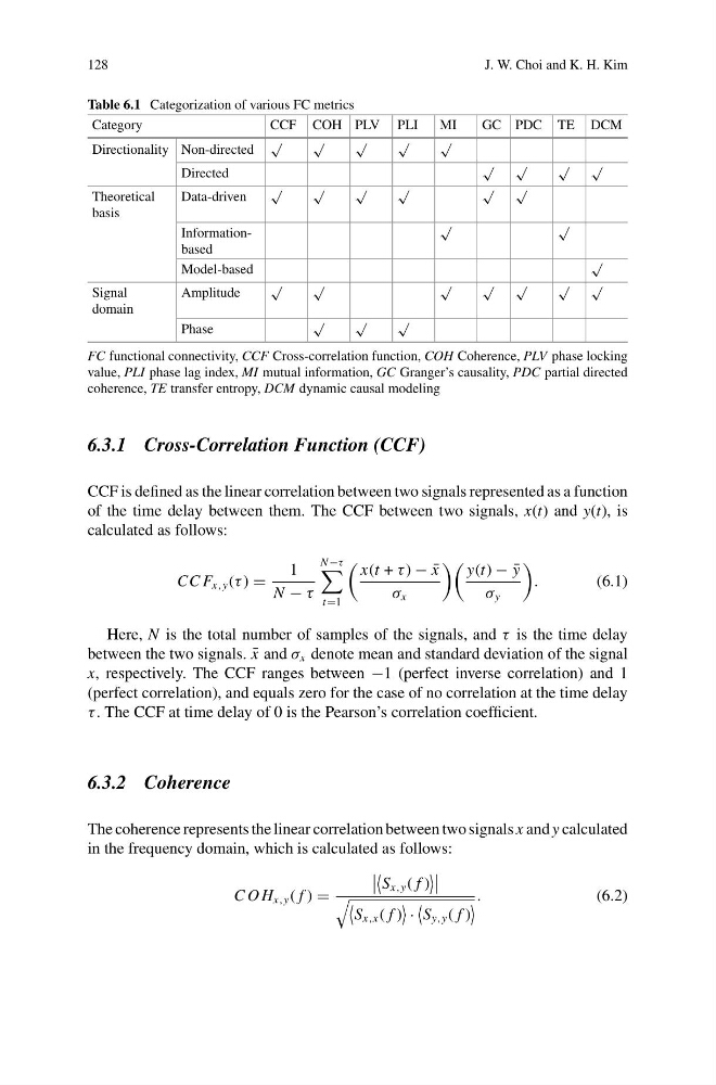
Table 6.1 Categorization of various FC metrics
Category
CCF COH PLV PLI
MI
GC PDC TE DCM
Directionality Non-directed
√
√
√
√
√
Directed
√
√
√
√
Theoretical
basis
Data-driven
√
√
√
√
√
√
Informationbased
√
√
Model-based
√
Signal
domain
Amplitude
√
√
√
√
√
√
√
Phase
√
√
√
FC functional connectivity, CCF Cross-correlation function, COH Coherence, PLV phase locking
value, PLI phase lag index, MI mutual information, GC Granger’s causality, PDC partial directed
coherence, TE transfer entropy, DCM dynamic causal modeling
6.3.1 Cross-Correlation Function (CCF)
CCF is defined as the linear correlation between two signals represented as a function
of the time delay between them. The CCF between two signals, x(t) and y(t), is
calculated as follows:
CC F x,y (τ )
1
N − τ
N −τ
t1
x(t + τ ) − ¯
x
σ x
y(t) − ¯
y
σ y
.
(6.1)
Here, N is the total number of samples of the signals, and τ is the time delay
between the two signals. ¯
x and σ x denote mean and standard deviation of the signal
x, respectively. The CCF ranges between −1 (perfect inverse correlation) and 1
(perfect correlation), and equals zero for the case of no correlation at the time delay
τ . The CCF at time delay of 0 is the Pearson’s correlation coefficient.
6.3.2 Coherence
The coherence represents the linear correlation between two signals x and y calculated
in the frequency domain, which is calculated as follows:
C O H x,y ( f )
S x,y ( f )
S x,x ( f )
·
S y,y ( f )
.
(6.2)
J. W. Choi and K. H. Kim
Table 6.1 Categorization of various FC metrics
Category
CCF COH PLV PLI
MI
GC PDC TE DCM
Directionality Non-directed
√
√
√
√
√
Directed
√
√
√
√
Theoretical
basis
Data-driven
√
√
√
√
√
√
Informationbased
√
√
Model-based
√
Signal
domain
Amplitude
√
√
√
√
√
√
√
Phase
√
√
√
FC functional connectivity, CCF Cross-correlation function, COH Coherence, PLV phase locking
value, PLI phase lag index, MI mutual information, GC Granger’s causality, PDC partial directed
coherence, TE transfer entropy, DCM dynamic causal modeling
6.3.1 Cross-Correlation Function (CCF)
CCF is defined as the linear correlation between two signals represented as a function
of the time delay between them. The CCF between two signals, x(t) and y(t), is
calculated as follows:
CC F x,y (τ )
1
N − τ
N −τ
t1
x(t + τ ) − ¯
x
σ x
y(t) − ¯
y
σ y
.
(6.1)
Here, N is the total number of samples of the signals, and τ is the time delay
between the two signals. ¯
x and σ x denote mean and standard deviation of the signal
x, respectively. The CCF ranges between −1 (perfect inverse correlation) and 1
(perfect correlation), and equals zero for the case of no correlation at the time delay
τ . The CCF at time delay of 0 is the Pearson’s correlation coefficient.
6.3.2 Coherence
The coherence represents the linear correlation between two signals x and y calculated
in the frequency domain, which is calculated as follows:
C O H x,y ( f )
S x,y ( f )
S x,x ( f )
·
S y,y ( f )
.
(6.2)