

5 EEG Source Imaging and Multimodal Neuroimaging
99
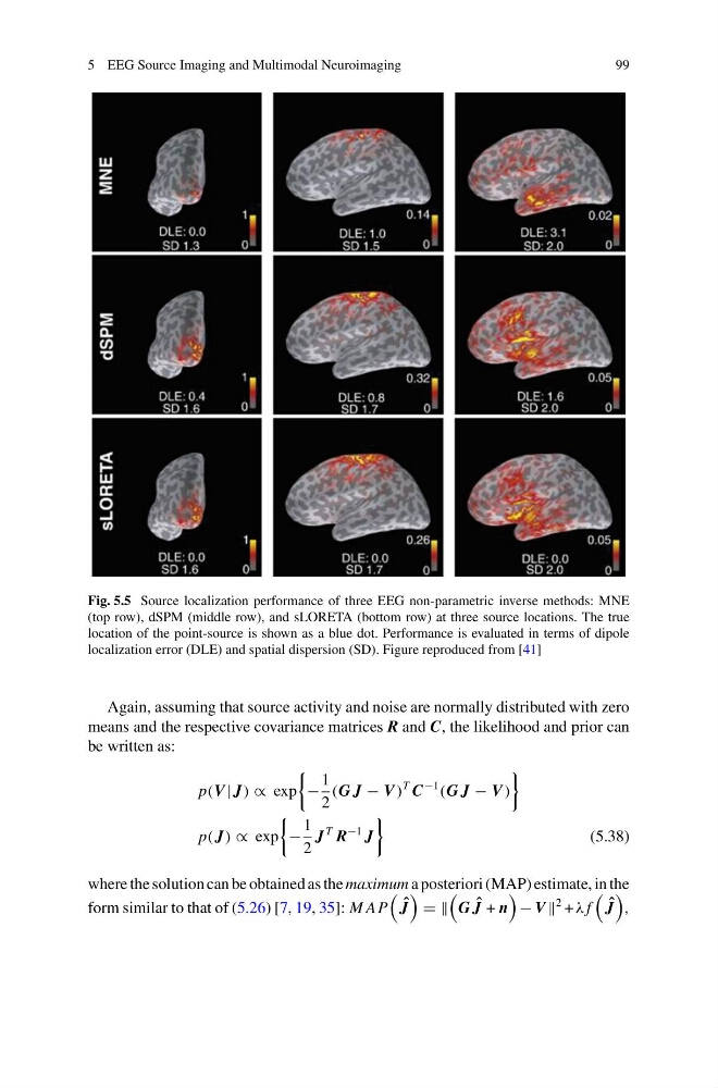
Fig. 5.5 Source localization performance of three EEG non-parametric inverse methods: MNE
(top row), dSPM (middle row), and sLORETA (bottom row) at three source locations. The true
location of the point-source is shown as a blue dot. Performance is evaluated in terms of dipole
localization error (DLE) and spatial dispersion (SD). Figure reproduced from [41]
Again, assuming that source activity and noise are normally distributed with zero
means and the respective covariance matrices R and C, the likelihood and prior can
be written as:
p(V | J) ∝ exp
−
1
2
(G J − V )
T C
−1
(G J − V )
p( J) ∝ exp
−
1
2
J
T R
−1 J
(5.38)
where the solution can be obtained as the maximum a posteriori (MAP) estimate, in the
form similar to that of (5.26) [7, 19, 35]: M AP
ˆ
J
G ˆ
J + n
− V
2 + λ f
ˆ
J
,
99
Fig. 5.5 Source localization performance of three EEG non-parametric inverse methods: MNE
(top row), dSPM (middle row), and sLORETA (bottom row) at three source locations. The true
location of the point-source is shown as a blue dot. Performance is evaluated in terms of dipole
localization error (DLE) and spatial dispersion (SD). Figure reproduced from [41]
Again, assuming that source activity and noise are normally distributed with zero
means and the respective covariance matrices R and C, the likelihood and prior can
be written as:
p(V | J) ∝ exp
−
1
2
(G J − V )
T C
−1
(G J − V )
p( J) ∝ exp
−
1
2
J
T R
−1 J
(5.38)
where the solution can be obtained as the maximum a posteriori (MAP) estimate, in the
form similar to that of (5.26) [7, 19, 35]: M AP
ˆ
J
G ˆ
J + n
− V
2 + λ f
ˆ
J
,