

98
Y. Zhang
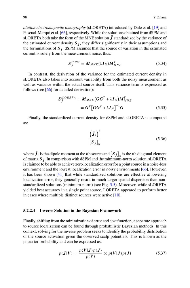
olution electromagnetic tomography (sLORETA) introduced by Dale et al. [19] and
Pascual-Marqui et al. [66], respectively. While the solutions obtained from dSPM and
sLORETA both take the form of the MNE solution ˆ
J standardized by the variance of
the estimated current density S ˆ
J , they differ significantly in their assumptions and
the formulations of S ˆ
J . dSPM assumes that the source of variation in the estimated
current is solely from the measurement noise, thus:
S
d S P M
ˆ
J
M M N E (λI N )M
T
M N E
(5.34)
In contrast, the derivation of the variance for the estimated current density in
sLORETA also takes into account variability from both the noisy measurement as
well as variance within the actual source itself. This variance term is expressed as
follows (see [66] for detailed derivation):
S
sL O R ET A
ˆ
J
M M N E
GG
T + λI N
M
T
M N E
G
T
GG
T + λI N
−1 G
(5.35)
Finally, the standardized current density for dSPM and sLORETA is computed
as:
ˆ
J i
2
S ˆ
J
ii
(5.36)
where ˆ
J i is the dipole moment at the ith source and
S ˆ
J
ii
is the ith diagonal element
of matrix S ˆ
J . In comparison with dSPM and the minimum-norm solution, sLORETA
is claimed to be able to achieve zero localization error for a point source in a noise-less
environment and the lowest localization error in noisy environments [66]. However,
it has been shown [41] that while standardized solutions are effective at lowering
localization error, they generally result in much larger spatial dispersion than nonstandardized solutions (minimum-norm) (see Fig. 5.5). Moreover, while sLORETA
yielded best accuracy in a single point source, LORETA appeared to perform better
in cases where multiple distinct sources were active [10].
5.2.2.4 Inverse Solution in the Bayesian Framework
Finally, shifting from the minimization of error and cost function, a separate approach
to source localization can be found through probabilistic Bayesian methods. In this
context, solving for the inverse problem seeks to identify the probability distribution
of the source activation given the observed scalp potentials. This is known as the
posterior probability and can be expressed as:
p( J|V )
p(V | J) p( J)
p(V )
∝ p(V | J) p( J)
(5.37)
Y. Zhang
olution electromagnetic tomography (sLORETA) introduced by Dale et al. [19] and
Pascual-Marqui et al. [66], respectively. While the solutions obtained from dSPM and
sLORETA both take the form of the MNE solution ˆ
J standardized by the variance of
the estimated current density S ˆ
J , they differ significantly in their assumptions and
the formulations of S ˆ
J . dSPM assumes that the source of variation in the estimated
current is solely from the measurement noise, thus:
S
d S P M
ˆ
J
M M N E (λI N )M
T
M N E
(5.34)
In contrast, the derivation of the variance for the estimated current density in
sLORETA also takes into account variability from both the noisy measurement as
well as variance within the actual source itself. This variance term is expressed as
follows (see [66] for detailed derivation):
S
sL O R ET A
ˆ
J
M M N E
GG
T + λI N
M
T
M N E
G
T
GG
T + λI N
−1 G
(5.35)
Finally, the standardized current density for dSPM and sLORETA is computed
as:
ˆ
J i
2
S ˆ
J
ii
(5.36)
where ˆ
J i is the dipole moment at the ith source and
S ˆ
J
ii
is the ith diagonal element
of matrix S ˆ
J . In comparison with dSPM and the minimum-norm solution, sLORETA
is claimed to be able to achieve zero localization error for a point source in a noise-less
environment and the lowest localization error in noisy environments [66]. However,
it has been shown [41] that while standardized solutions are effective at lowering
localization error, they generally result in much larger spatial dispersion than nonstandardized solutions (minimum-norm) (see Fig. 5.5). Moreover, while sLORETA
yielded best accuracy in a single point source, LORETA appeared to perform better
in cases where multiple distinct sources were active [10].
5.2.2.4 Inverse Solution in the Bayesian Framework
Finally, shifting from the minimization of error and cost function, a separate approach
to source localization can be found through probabilistic Bayesian methods. In this
context, solving for the inverse problem seeks to identify the probability distribution
of the source activation given the observed scalp potentials. This is known as the
posterior probability and can be expressed as:
p( J|V )
p(V | J) p( J)
p(V )
∝ p(V | J) p( J)
(5.37)