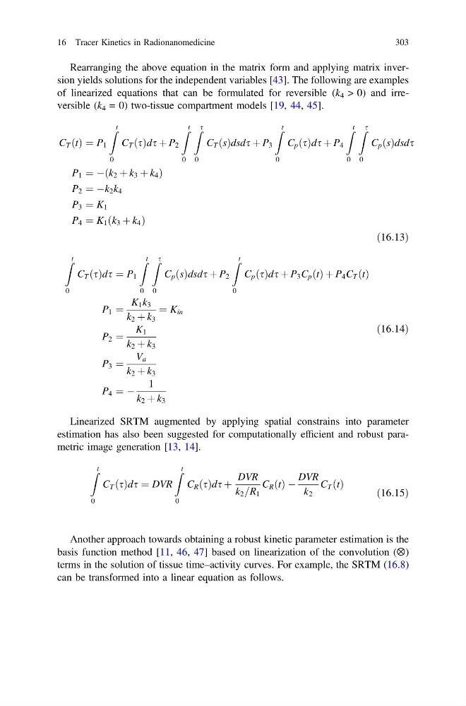
Rearranging the above equation in the matrix form and applying matrix inversion yields solutions for the independent variables [43]. The following are examples
of linearized equations that can be formulated for reversible (k 4 > 0) and irreversible (k 4 = 0) two-tissue compartment models [19, 44, 45].
C T ðtÞ ¼ P 1
Z t
0
C T ðsÞds þ P 2
Z t
0
Z s
0
C T ðsÞdsds þ P 3
Z t
0
C p ðsÞds þ P 4
Z t
0
Z s
0
C p ðsÞdsds
P 1 ¼ Àðk 2 þ k 3 þ k 4 Þ
P 2 ¼ Àk 2 k 4
P 3 ¼ K 1
P 4 ¼ K 1 ðk 3 þ k 4 Þ
ð16:13Þ
Z t
0
C T ðsÞds ¼ P 1
Z t
0
Z s
0
C p ðsÞdsds þ P 2
Z t
0
C p ðsÞds þ P 3 C p ðtÞ þ P 4 C T ðtÞ
P 1 ¼
K 1 k 3
k 2 þ k 3
¼ K in
P 2 ¼
K 1
k 2 þ k 3
P 3 ¼
V a
k 2 þ k 3
P 4 ¼ À
1
k 2 þ k 3
ð16:14Þ
Linearized SRTM augmented by applying spatial constrains into parameter
estimation has also been suggested for computationally efficient and robust parametric image generation [13, 14].
Z t
0
C T ðsÞds ¼ DVR
Z t
0
C R ðsÞds þ
DVR
k 2 =R 1
C R ðtÞ À
DVR
k 2
C T ðtÞ
ð16:15Þ
Another approach towards obtaining a robust kinetic parameter estimation is the
basis function method [11, 46, 47] based on linearization of the convolution (⊗)
terms in the solution of tissue time–activity curves. For example, the SRTM (16.8)
can be transformed into a linear equation as follows.
16 Tracer Kinetics in Radionanomedicine
303