

16.4 Parameter Estimation
Noise in the tissue time–activity curve and input function leads to bias and a
variation in the estimated kinetic parameters. Usually, this bias and variation
increase as the noise level becomes higher (Fig. 16.3). Nonlinear parameter estimation based on an iterative search of the final solution is vulnerable to noise, as
noise generates a local minima in the parameter search space. As such, one needs to
assign proper initial values relatively close to the final solution to avoid convergence to the local minima. Constraints in the bounds of estimates and some regularizations based on prior knowledge regarding the properties of radiotracers are
sometimes helpful in finding the best solution.
The parameter estimation procedure can be simplified by transforming the differential equations of the kinetic model into a linearized form. Several different
graphical analysis (GA) methods based on simple linear regression models are
available. Two most popular GA methods comprise the Gjedde–Patlak plot for an
irreversible system [34–36] and the Logan plot for a reversible one [37, 38].
Additionally, methods like the relative equilibrium-based graphical method for
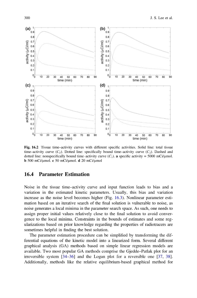
Fig. 16.2 Tissue time–activity curves with different specific activities. Solid line: total tissue
time–activity curve (C T ). Dotted line: specifically bound time–activity curve (C 2 ). Dashed and
dotted line: nonspecifically bound time–activity curve (C 1 ). a specific activity = 5000 mCi/µmol.
b 500 mCi/µmol. c 50 mCi/µmol. d 20 mCi/µmol
300
J. S. Lee et al.
Noise in the tissue time–activity curve and input function leads to bias and a
variation in the estimated kinetic parameters. Usually, this bias and variation
increase as the noise level becomes higher (Fig. 16.3). Nonlinear parameter estimation based on an iterative search of the final solution is vulnerable to noise, as
noise generates a local minima in the parameter search space. As such, one needs to
assign proper initial values relatively close to the final solution to avoid convergence to the local minima. Constraints in the bounds of estimates and some regularizations based on prior knowledge regarding the properties of radiotracers are
sometimes helpful in finding the best solution.
The parameter estimation procedure can be simplified by transforming the differential equations of the kinetic model into a linearized form. Several different
graphical analysis (GA) methods based on simple linear regression models are
available. Two most popular GA methods comprise the Gjedde–Patlak plot for an
irreversible system [34–36] and the Logan plot for a reversible one [37, 38].
Additionally, methods like the relative equilibrium-based graphical method for
Fig. 16.2 Tissue time–activity curves with different specific activities. Solid line: total tissue
time–activity curve (C T ). Dotted line: specifically bound time–activity curve (C 2 ). Dashed and
dotted line: nonspecifically bound time–activity curve (C 1 ). a specific activity = 5000 mCi/µmol.
b 500 mCi/µmol. c 50 mCi/µmol. d 20 mCi/µmol
300
J. S. Lee et al.