

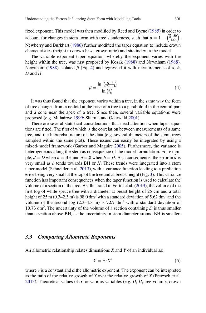
fixed exponent. This model was then modified by Reed and Byrne (1985) in order to
account for changes in stem form with tree slenderness, such that β ¼ 1 À
H
D À30
120
.
Newberry and Burkhart (1986) further modified the taper equation to include crown
characteristics (height to crown base, crown ratio) and site index in the model.
The variable exponent taper equation, whereby the exponent varies with the
height within the tree, was first proposed by Kozak (1988) and Newnham (1988).
Newnham (1988) isolated β (Eq. 4) and regressed it with measurements of d, h,
D and H.
β ¼
ln
HÀh
HÀBH
À
Á
ln
d
D
À Á
ð4Þ
It was thus found that the exponent varies within a tree, in the same way the form
of tree changes from a neiloid at the base of a tree to a paraboloid in the central part
and a cone near the apex of a tree. Since then, several variable equations were
proposed (e.g. Muhairwe 1999; Sharma and Oderwald 2001).
There are several statistical considerations that need attention when taper equations are fitted. The first of which is the correlation between measurements of a same
tree, and the hierarchal nature of the data (e.g. several diameters of the stem, trees
sampled within the same plot). These issues can easily be integrated by using a
mixed-model framework (Garber and Maguire 2005). Furthermore, the variance is
heterogeneous along the stem as consequence of the model formulation. For example, d ¼ D when h ¼ BH and d ¼ 0 when h ¼ H. As a consequence, the error in b
d is
very small as h tends towards BH or H. These trends were integrated into a stem
taper model (Schneider et al. 2013), with a variance function leading to a prediction
error being very small at the top of the tree and at breast height (Fig. 3). This variance
function has important consequences when the taper function is used to calculate the
volume of a section of the tree. As illustrated in Fortin et al. (2013), the volume of the
first log of white spruce tree with a diameter at breast height of 25 cm and a total
height of 25 m (0.3–2.3 m) is 98.0 dm
3 with a standard deviation of 5.62 dm
3 and the
volume of the second log (2.3–4.3 m) is 72.7 dm
3 with a standard deviation of
10.73 dm
3 . The uncertainty of the volume of a section containing D is thus smaller
than a section above BH, as the uncertainty in stem diameter around BH is smaller.
3.3 Comparing Allometric Exponents
An allometric relationship relates dimensions X and Y of an individual as:
Y ¼ c ∙ X
α
ð5Þ
where c is a constant and α the allometric exponent. The exponent can be interpreted
as the ratio of the relative growth of Y over the relative growth of X (Pretzsch et al.
2013). Theoretical values of α for various variables (e.g. D, H, tree volume, crown
Understanding the Factors Influencing Stem Form with Modelling Tools
301
account for changes in stem form with tree slenderness, such that β ¼ 1 À
H
D À30
120
.
Newberry and Burkhart (1986) further modified the taper equation to include crown
characteristics (height to crown base, crown ratio) and site index in the model.
The variable exponent taper equation, whereby the exponent varies with the
height within the tree, was first proposed by Kozak (1988) and Newnham (1988).
Newnham (1988) isolated β (Eq. 4) and regressed it with measurements of d, h,
D and H.
β ¼
ln
HÀh
HÀBH
À
Á
ln
d
D
À Á
ð4Þ
It was thus found that the exponent varies within a tree, in the same way the form
of tree changes from a neiloid at the base of a tree to a paraboloid in the central part
and a cone near the apex of a tree. Since then, several variable equations were
proposed (e.g. Muhairwe 1999; Sharma and Oderwald 2001).
There are several statistical considerations that need attention when taper equations are fitted. The first of which is the correlation between measurements of a same
tree, and the hierarchal nature of the data (e.g. several diameters of the stem, trees
sampled within the same plot). These issues can easily be integrated by using a
mixed-model framework (Garber and Maguire 2005). Furthermore, the variance is
heterogeneous along the stem as consequence of the model formulation. For example, d ¼ D when h ¼ BH and d ¼ 0 when h ¼ H. As a consequence, the error in b
d is
very small as h tends towards BH or H. These trends were integrated into a stem
taper model (Schneider et al. 2013), with a variance function leading to a prediction
error being very small at the top of the tree and at breast height (Fig. 3). This variance
function has important consequences when the taper function is used to calculate the
volume of a section of the tree. As illustrated in Fortin et al. (2013), the volume of the
first log of white spruce tree with a diameter at breast height of 25 cm and a total
height of 25 m (0.3–2.3 m) is 98.0 dm
3 with a standard deviation of 5.62 dm
3 and the
volume of the second log (2.3–4.3 m) is 72.7 dm
3 with a standard deviation of
10.73 dm
3 . The uncertainty of the volume of a section containing D is thus smaller
than a section above BH, as the uncertainty in stem diameter around BH is smaller.
3.3 Comparing Allometric Exponents
An allometric relationship relates dimensions X and Y of an individual as:
Y ¼ c ∙ X
α
ð5Þ
where c is a constant and α the allometric exponent. The exponent can be interpreted
as the ratio of the relative growth of Y over the relative growth of X (Pretzsch et al.
2013). Theoretical values of α for various variables (e.g. D, H, tree volume, crown
Understanding the Factors Influencing Stem Form with Modelling Tools
301