

where Г is Kirchoff matrix obtained by GNM. The average hit time
for the i-th residue is the average of H(i, j) over all starting
points i. The commute time is defined by the sum of the hitting
times in both directions, that is:
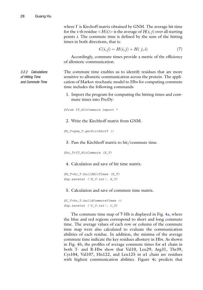
C i, j
ð Þ ¼ H i, j
ð Þ þ H j, i
ð
Þ
ð7Þ
Accordingly, commute times provide a metric of the efficiency
of allosteric communication.
3.2.2 Calculations
of Hitting Time
and Commute Time
The commute time enables us to identify residues that are more
sensitive to allosteric communication across the protein. The application of Markov stochastic model to Hbs for computing commute
time includes the following commands:
1. Import the program for computing the hitting times and commute times into ProDy:
$from IT_HitCommute import *
2. Write the Kirchhoff matrix from GNM.
$K_T=gnm_T.getKirchhoff ()
3. Pass the Kirchhoff matrix to hit/commute time.
$hc_T=IT_HitCommute (K_T)
4. Calculation and save of hit time matrix.
$H_T=hc_T.buildHitTimes (K_T)
$np.savetxt (‘H_T.txt’, H_T)
5. Calculation and save of commute time matrix.
$C_T=hc_T.buildCommuteTimes ()
$np.savetxt (‘C_T.txt’, C_T)
The commute time map of ?-Hb is displayed in Fig. 4a, where
the blue and red regions correspond to short and long commute
time. The average values of each row or column of the commute
time map were also calculated to evaluate the communication
abilities of each residue. In addition, the minima of the average
commute time indicate the key residues allostery in Hbs. As shown
in Fig. 4b, the profiles of average commute times for α1 chain in
both T- and R-Hbs show that Val10, Leu29, Arg31, Thr39,
Cys104, Val107, His122, and Leu125 in α1 chain are residues
with highest communication abilities. Figure 4c predicts that
28
Guang Hu
for the i-th residue
points i. The commute time is defined by the sum of the hitting
times in both directions, that is:
C i, j
ð Þ ¼ H i, j
ð Þ þ H j, i
ð
Þ
ð7Þ
Accordingly, commute times provide a metric of the efficiency
of allosteric communication.
3.2.2 Calculations
of Hitting Time
and Commute Time
The commute time enables us to identify residues that are more
sensitive to allosteric communication across the protein. The application of Markov stochastic model to Hbs for computing commute
time includes the following commands:
1. Import the program for computing the hitting times and commute times into ProDy:
$from IT_HitCommute import *
2. Write the Kirchhoff matrix from GNM.
$K_T=gnm_T.getKirchhoff ()
3. Pass the Kirchhoff matrix to hit/commute time.
$hc_T=IT_HitCommute (K_T)
4. Calculation and save of hit time matrix.
$H_T=hc_T.buildHitTimes (K_T)
$np.savetxt (‘H_T.txt’, H_T)
5. Calculation and save of commute time matrix.
$C_T=hc_T.buildCommuteTimes ()
$np.savetxt (‘C_T.txt’, C_T)
The commute time map of ?-Hb is displayed in Fig. 4a, where
the blue and red regions correspond to short and long commute
time. The average values of each row or column of the commute
time map were also calculated to evaluate the communication
abilities of each residue. In addition, the minima of the average
commute time indicate the key residues allostery in Hbs. As shown
in Fig. 4b, the profiles of average commute times for α1 chain in
both T- and R-Hbs show that Val10, Leu29, Arg31, Thr39,
Cys104, Val107, His122, and Leu125 in α1 chain are residues
with highest communication abilities. Figure 4c predicts that
28
Guang Hu