

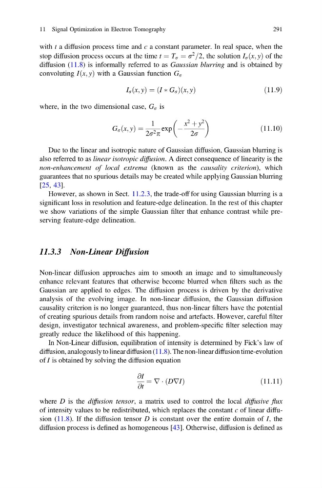
with t a diffusion process time and c a constant parameter. In real space, when the
stop diffusion process occurs at the time t ¼ T r ¼ r
2
=2, the solution I r ðx; yÞ of the
diffusion (11.8) is informally referred to as Gaussian blurring and is obtained by
convoluting Iðx; yÞ with a Gaussian function G r
I r ðx; yÞ ¼ ðI Ã G r Þðx; yÞ
ð 11:9Þ
where, in the two dimensional case, G r is
G r ðx; yÞ ¼
1
2r 2 p
exp À
x
2
þ y
2
2r
ð11:10Þ
Due to the linear and isotropic nature of Gaussian diffusion, Gaussian blurring is
also referred to as linear isotropic diffusion. A direct consequence of linearity is the
non-enhancement of local extrema (known as the causality criterion), which
guarantees that no spurious details may be created while applying Gaussian blurring
[25, 43].
However, as shown in Sect. 11.2.3, the trade-off for using Gaussian blurring is a
significant loss in resolution and feature-edge delineation. In the rest of this chapter
we show variations of the simple Gaussian filter that enhance contrast while preserving feature-edge delineation.
11.3.3 Non-Linear Diffusion
Non-linear diffusion approaches aim to smooth an image and to simultaneously
enhance relevant features that otherwise become blurred when filters such as the
Gaussian are applied to edges. The diffusion process is driven by the derivative
analysis of the evolving image. In non-linear diffusion, the Gaussian diffusion
causality criterion is no longer guaranteed, thus non-linear filters have the potential
of creating spurious details from random noise and artefacts. However, careful filter
design, investigator technical awareness, and problem-specific filter selection may
greatly reduce the likelihood of this happening.
In Non-Linear diffusion, equilibration of intensity is determined by Fick’s law of
diffusion, analogously to linear diffusion (11.8). The non-linear diffusion time-evolution
of I is obtained by solving the diffusion equation
@I
@t
¼ r Á ðDrIÞ
ð 11:11Þ
where D is the diffusion tensor, a matrix used to control the local diffusive flux
of intensity values to be redistributed, which replaces the constant c of linear diffusion (11.8). If the diffusion tensor D is constant over the entire domain of I, the
diffusion process is defined as homogeneous [43]. Otherwise, diffusion is defined as
11 Signal Optimization in Electron Tomography
291
stop diffusion process occurs at the time t ¼ T r ¼ r
2
=2, the solution I r ðx; yÞ of the
diffusion (11.8) is informally referred to as Gaussian blurring and is obtained by
convoluting Iðx; yÞ with a Gaussian function G r
I r ðx; yÞ ¼ ðI Ã G r Þðx; yÞ
ð 11:9Þ
where, in the two dimensional case, G r is
G r ðx; yÞ ¼
1
2r 2 p
exp À
x
2
þ y
2
2r
ð11:10Þ
Due to the linear and isotropic nature of Gaussian diffusion, Gaussian blurring is
also referred to as linear isotropic diffusion. A direct consequence of linearity is the
non-enhancement of local extrema (known as the causality criterion), which
guarantees that no spurious details may be created while applying Gaussian blurring
[25, 43].
However, as shown in Sect. 11.2.3, the trade-off for using Gaussian blurring is a
significant loss in resolution and feature-edge delineation. In the rest of this chapter
we show variations of the simple Gaussian filter that enhance contrast while preserving feature-edge delineation.
11.3.3 Non-Linear Diffusion
Non-linear diffusion approaches aim to smooth an image and to simultaneously
enhance relevant features that otherwise become blurred when filters such as the
Gaussian are applied to edges. The diffusion process is driven by the derivative
analysis of the evolving image. In non-linear diffusion, the Gaussian diffusion
causality criterion is no longer guaranteed, thus non-linear filters have the potential
of creating spurious details from random noise and artefacts. However, careful filter
design, investigator technical awareness, and problem-specific filter selection may
greatly reduce the likelihood of this happening.
In Non-Linear diffusion, equilibration of intensity is determined by Fick’s law of
diffusion, analogously to linear diffusion (11.8). The non-linear diffusion time-evolution
of I is obtained by solving the diffusion equation
@I
@t
¼ r Á ðDrIÞ
ð 11:11Þ
where D is the diffusion tensor, a matrix used to control the local diffusive flux
of intensity values to be redistributed, which replaces the constant c of linear diffusion (11.8). If the diffusion tensor D is constant over the entire domain of I, the
diffusion process is defined as homogeneous [43]. Otherwise, diffusion is defined as
11 Signal Optimization in Electron Tomography
291