

6 Identity by Descent in the Mapping of Genetic Traits
151
population there is no such framework. However, just as in an association test, permutation of case-control labels provides a null distribution of the test statistic (6.15)
under which there is no association between IBD at the test location and the casecontrol status of individuals. Since IBD is on a scale of Mbp, at most 3,000 tests can
cover the genome. This results in a multiple testing burden that is several orders of
magnitude less than that for SNP based GWAS.
To show that population-based IBD mapping can work, we present the details of
part of the study undertaken by Browning and Thompson (2012). A coalescent
simulation including selection and mutation provided a base population with
effective size N e = 10 4 , over a 200 kbp region of chromosome, representing a
functional gene region. The population was then run forward, and, at some later
time point, IBD relative to the base population was scored in descendant individuals.
In the example summarized here, the effective size of the recent population was
N e = 10 5 and the time-depth of IBD was G = 25 generations.
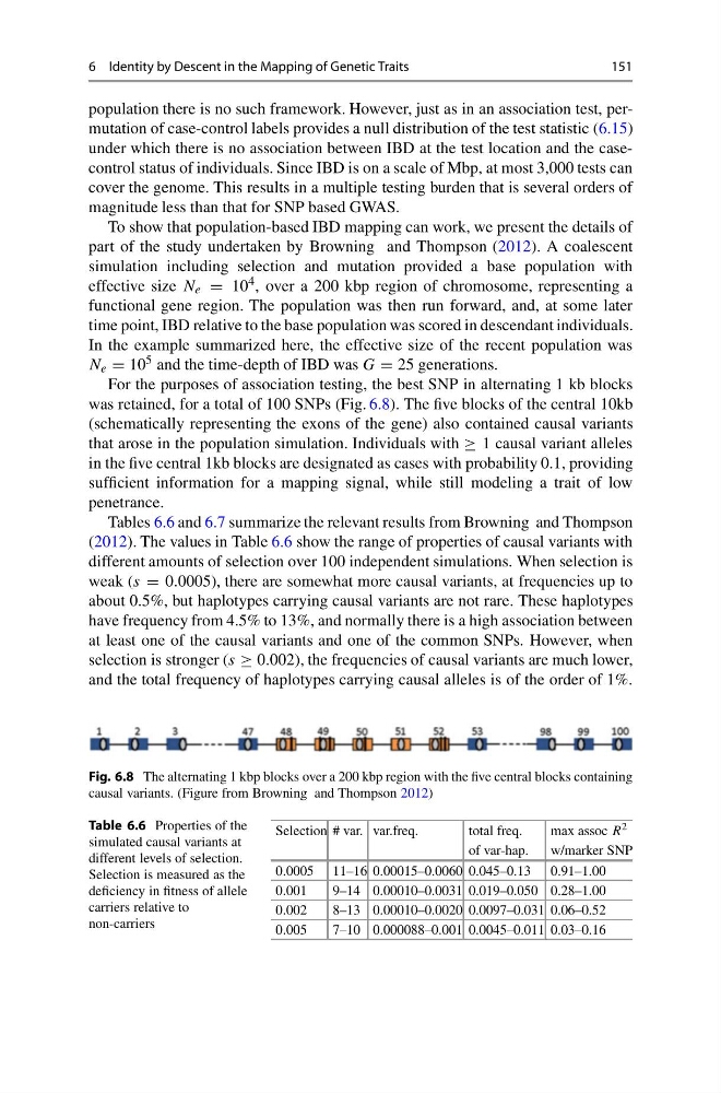
For the purposes of association testing, the best SNP in alternating 1 kb blocks
was retained, for a total of 100 SNPs (Fig. 6.8). The five blocks of the central 10kb
(schematically representing the exons of the gene) also contained causal variants
that arose in the population simulation. Individuals with ≥ 1 causal variant alleles
in the five central 1kb blocks are designated as cases with probability 0.1, providing
sufficient information for a mapping signal, while still modeling a trait of low
penetrance.
Tables 6.6 and 6.7 summarize the relevant results from Browning and Thompson
(2012). The values in Table 6.6 show the range of properties of causal variants with
different amounts of selection over 100 independent simulations. When selection is
weak (s = 0.0005), there are somewhat more causal variants, at frequencies up to
about 0.5%, but haplotypes carrying causal variants are not rare. These haplotypes
have frequency from 4.5% to 13%, and normally there is a high association between
at least one of the causal variants and one of the common SNPs. However, when
selection is stronger (s ≥ 0.002), the frequencies of causal variants are much lower,
and the total frequency of haplotypes carrying causal alleles is of the order of 1%.
Fig. 6.8 The alternating 1 kbp blocks over a 200 kbp region with the five central blocks containing
causal variants. (Figure from Browning and Thompson 2012)
Table 6.6 Properties of the
simulated causal variants at
different levels of selection.
Selection is measured as the
deficiency in fitness of allele
carriers relative to
non-carriers
Selection # var. var.freq.
total freq.
max assoc R 2
of var-hap.
w/marker SNP
0.0005 11–16 0.00015–0.0060 0.045–0.13 0.91–1.00
0.001
9–14 0.00010–0.0031 0.019–0.050 0.28–1.00
0.002
8–13 0.00010–0.0020 0.0097–0.031 0.06–0.52
0.005
7–10 0.000088–0.001 0.0045–0.011 0.03–0.16
151
population there is no such framework. However, just as in an association test, permutation of case-control labels provides a null distribution of the test statistic (6.15)
under which there is no association between IBD at the test location and the casecontrol status of individuals. Since IBD is on a scale of Mbp, at most 3,000 tests can
cover the genome. This results in a multiple testing burden that is several orders of
magnitude less than that for SNP based GWAS.
To show that population-based IBD mapping can work, we present the details of
part of the study undertaken by Browning and Thompson (2012). A coalescent
simulation including selection and mutation provided a base population with
effective size N e = 10 4 , over a 200 kbp region of chromosome, representing a
functional gene region. The population was then run forward, and, at some later
time point, IBD relative to the base population was scored in descendant individuals.
In the example summarized here, the effective size of the recent population was
N e = 10 5 and the time-depth of IBD was G = 25 generations.
For the purposes of association testing, the best SNP in alternating 1 kb blocks
was retained, for a total of 100 SNPs (Fig. 6.8). The five blocks of the central 10kb
(schematically representing the exons of the gene) also contained causal variants
that arose in the population simulation. Individuals with ≥ 1 causal variant alleles
in the five central 1kb blocks are designated as cases with probability 0.1, providing
sufficient information for a mapping signal, while still modeling a trait of low
penetrance.
Tables 6.6 and 6.7 summarize the relevant results from Browning and Thompson
(2012). The values in Table 6.6 show the range of properties of causal variants with
different amounts of selection over 100 independent simulations. When selection is
weak (s = 0.0005), there are somewhat more causal variants, at frequencies up to
about 0.5%, but haplotypes carrying causal variants are not rare. These haplotypes
have frequency from 4.5% to 13%, and normally there is a high association between
at least one of the causal variants and one of the common SNPs. However, when
selection is stronger (s ≥ 0.002), the frequencies of causal variants are much lower,
and the total frequency of haplotypes carrying causal alleles is of the order of 1%.
Fig. 6.8 The alternating 1 kbp blocks over a 200 kbp region with the five central blocks containing
causal variants. (Figure from Browning and Thompson 2012)
Table 6.6 Properties of the
simulated causal variants at
different levels of selection.
Selection is measured as the
deficiency in fitness of allele
carriers relative to
non-carriers
Selection # var. var.freq.
total freq.
max assoc R 2
of var-hap.
w/marker SNP
0.0005 11–16 0.00015–0.0060 0.045–0.13 0.91–1.00
0.001
9–14 0.00010–0.0031 0.019–0.050 0.28–1.00
0.002
8–13 0.00010–0.0020 0.0097–0.031 0.06–0.52
0.005
7–10 0.000088–0.001 0.0045–0.011 0.03–0.16