

6 Identity by Descent in the Mapping of Genetic Traits
149
where the expectation is over the values of Z(λ) given X. The methods of Sect. 6.3.2
allow a large number, N, of patterns of IBD Z (k) (k = 1, . . . , N) across the
chromosome to be sampled jointly for all relevant locations j in any collection
of models {λ : λ ⊂ conditional on the joint marker data on individuals and
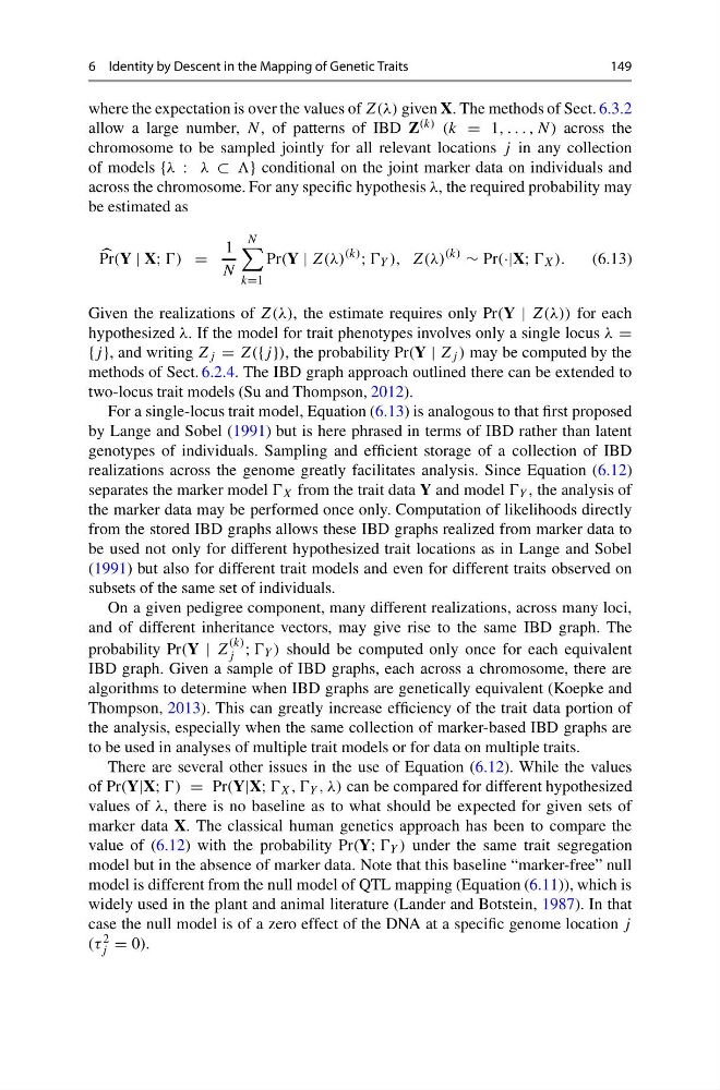
across the chromosome. For any specific hypothesis λ, the required probability may
be estimated as
Pr(Y | X; =
1
N
N
k=1
Pr(Y | Z(λ)
(k)
; Y ), Z(λ)
(k)
∼ Pr(·|X; X ).
(6.13)
Given the realizations of Z(λ), the estimate requires only Pr(Y | Z(λ)) for each
hypothesized λ. If the model for trait phenotypes involves only a single locus λ =
{j }, and writing Z j = Z({j }), the probability Pr(Y | Z j ) may be computed by the
methods of Sect. 6.2.4. The IBD graph approach outlined there can be extended to
two-locus trait models (Su and Thompson, 2012).
For a single-locus trait model, Equation (6.13) is analogous to that first proposed
by Lange and Sobel (1991) but is here phrased in terms of IBD rather than latent
genotypes of individuals. Sampling and efficient storage of a collection of IBD
realizations across the genome greatly facilitates analysis. Since Equation (6.12)
separates the marker model X from the trait data Y and model Y , the analysis of
the marker data may be performed once only. Computation of likelihoods directly
from the stored IBD graphs allows these IBD graphs realized from marker data to
be used not only for different hypothesized trait locations as in Lange and Sobel
(1991) but also for different trait models and even for different traits observed on
subsets of the same set of individuals.
On a given pedigree component, many different realizations, across many loci,
and of different inheritance vectors, may give rise to the same IBD graph. The
probability Pr(Y | Z
(k)
j ; Y ) should be computed only once for each equivalent
IBD graph. Given a sample of IBD graphs, each across a chromosome, there are
algorithms to determine when IBD graphs are genetically equivalent (Koepke and
Thompson, 2013). This can greatly increase efficiency of the trait data portion of
the analysis, especially when the same collection of marker-based IBD graphs are
to be used in analyses of multiple trait models or for data on multiple traits.
There are several other issues in the use of Equation (6.12). While the values
of Pr(Y|X; = Pr(Y|X; X , , Y , λ) can be compared for different hypothesized
values of λ, there is no baseline as to what should be expected for given sets of
marker data X. The classical human genetics approach has been to compare the
value of (6.12) with the probability Pr(Y; Y ) under the same trait segregation
model but in the absence of marker data. Note that this baseline “marker-free” null
model is different from the null model of QTL mapping (Equation (6.11)), which is
widely used in the plant and animal literature (Lander and Botstein, 1987). In that
case the null model is of a zero effect of the DNA at a specific genome location j
(τ 2
j = 0).
149
where the expectation is over the values of Z(λ) given X. The methods of Sect. 6.3.2
allow a large number, N, of patterns of IBD Z (k) (k = 1, . . . , N) across the
chromosome to be sampled jointly for all relevant locations j in any collection
of models {λ : λ ⊂ conditional on the joint marker data on individuals and
across the chromosome. For any specific hypothesis λ, the required probability may
be estimated as
Pr(Y | X; =
1
N
N
k=1
Pr(Y | Z(λ)
(k)
; Y ), Z(λ)
(k)
∼ Pr(·|X; X ).
(6.13)
Given the realizations of Z(λ), the estimate requires only Pr(Y | Z(λ)) for each
hypothesized λ. If the model for trait phenotypes involves only a single locus λ =
{j }, and writing Z j = Z({j }), the probability Pr(Y | Z j ) may be computed by the
methods of Sect. 6.2.4. The IBD graph approach outlined there can be extended to
two-locus trait models (Su and Thompson, 2012).
For a single-locus trait model, Equation (6.13) is analogous to that first proposed
by Lange and Sobel (1991) but is here phrased in terms of IBD rather than latent
genotypes of individuals. Sampling and efficient storage of a collection of IBD
realizations across the genome greatly facilitates analysis. Since Equation (6.12)
separates the marker model X from the trait data Y and model Y , the analysis of
the marker data may be performed once only. Computation of likelihoods directly
from the stored IBD graphs allows these IBD graphs realized from marker data to
be used not only for different hypothesized trait locations as in Lange and Sobel
(1991) but also for different trait models and even for different traits observed on
subsets of the same set of individuals.
On a given pedigree component, many different realizations, across many loci,
and of different inheritance vectors, may give rise to the same IBD graph. The
probability Pr(Y | Z
(k)
j ; Y ) should be computed only once for each equivalent
IBD graph. Given a sample of IBD graphs, each across a chromosome, there are
algorithms to determine when IBD graphs are genetically equivalent (Koepke and
Thompson, 2013). This can greatly increase efficiency of the trait data portion of
the analysis, especially when the same collection of marker-based IBD graphs are
to be used in analyses of multiple trait models or for data on multiple traits.
There are several other issues in the use of Equation (6.12). While the values
of Pr(Y|X; = Pr(Y|X; X , , Y , λ) can be compared for different hypothesized
values of λ, there is no baseline as to what should be expected for given sets of
marker data X. The classical human genetics approach has been to compare the
value of (6.12) with the probability Pr(Y; Y ) under the same trait segregation
model but in the absence of marker data. Note that this baseline “marker-free” null
model is different from the null model of QTL mapping (Equation (6.11)), which is
widely used in the plant and animal literature (Lander and Botstein, 1987). In that
case the null model is of a zero effect of the DNA at a specific genome location j
(τ 2
j = 0).