

148
E. A. Thompson
between these two groups. For a quantitative trait, or when a more general trait
model is desired, it is more natural to consider Y given X. The same applies to IBDbased genetic mapping, where the marker data X are used to provide information
about IBD, Z. In the analogue of population-based association tests, we consider
differences in inferred IBD in pairs conditional on their trait status (see Sect. 6.4.3
below). In QTL mapping we model Y given the inferred IBD as in Equation (6.10)
above. In this section, we consider more generally the probability Pr(Y|X) in the
case where the pedigree structure is known.
As in classical linkage analysis (Smith, 1953; Morton, 1955), the goal is to test
for dependence between inheritance of DNA at specific genome locations and the
inheritance of DNA underlying a trait. The pedigree relationships among individuals
are assumed known, and genetic marker data X are available for some individuals,
for markers with known locations in the genome. Trait data Y are also available, and
a model is assumed for the relationship between the allelic type of latent causal DNA
and the trait of interest. In the following, X will denote the probability model for
the marker data X, which involves marker allele frequencies and locations which
are assumed known, and Y will denote the model for the trait, which specifies
frequencies of trait alleles, and the probabilities of phenotypes given latent trait
genotypes. The parameter λ is a set of locations at which, with any model, there is
hypothesized to be causal DNA. The full model is = (( X , , Y , λ). The full set of
all locations at which causal DNA is hypothesized in any model to be considered
will be denoted ; each λ is a subset of . For models with a single trait locus,
λ = {j } and is the set of j at which likelihoods are to be computed.
As before, we assume that Y and X are conditionally independent given Z and
denote by Z(λ) the IBD jointly at locations specified by λ. For single-locus trait
models λ = {j }, we write Z(λ) = Z j . Then
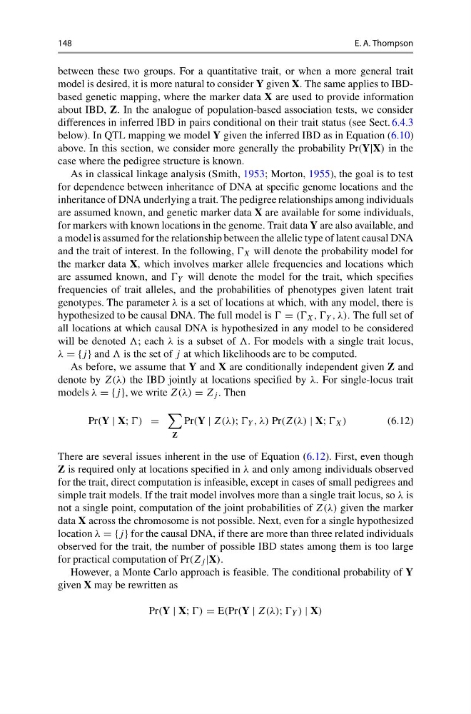
Pr(Y | X; =
Z
Pr(Y | Z(λ); Y , λ) Pr(Z(λ) | X; X )
(6.12)
There are several issues inherent in the use of Equation (6.12). First, even though
Z is required only at locations specified in λ and only among individuals observed
for the trait, direct computation is infeasible, except in cases of small pedigrees and
simple trait models. If the trait model involves more than a single trait locus, so λ is
not a single point, computation of the joint probabilities of Z(λ) given the marker
data X across the chromosome is not possible. Next, even for a single hypothesized
location λ = {j } for the causal DNA, if there are more than three related individuals
observed for the trait, the number of possible IBD states among them is too large
for practical computation of Pr(Z j |X).
However, a Monte Carlo approach is feasible. The conditional probability of Y
given X may be rewritten as
Pr(Y | X; = E(Pr(Y | Z(λ); Y ) | X)
E. A. Thompson
between these two groups. For a quantitative trait, or when a more general trait
model is desired, it is more natural to consider Y given X. The same applies to IBDbased genetic mapping, where the marker data X are used to provide information
about IBD, Z. In the analogue of population-based association tests, we consider
differences in inferred IBD in pairs conditional on their trait status (see Sect. 6.4.3
below). In QTL mapping we model Y given the inferred IBD as in Equation (6.10)
above. In this section, we consider more generally the probability Pr(Y|X) in the
case where the pedigree structure is known.
As in classical linkage analysis (Smith, 1953; Morton, 1955), the goal is to test
for dependence between inheritance of DNA at specific genome locations and the
inheritance of DNA underlying a trait. The pedigree relationships among individuals
are assumed known, and genetic marker data X are available for some individuals,
for markers with known locations in the genome. Trait data Y are also available, and
a model is assumed for the relationship between the allelic type of latent causal DNA
and the trait of interest. In the following, X will denote the probability model for
the marker data X, which involves marker allele frequencies and locations which
are assumed known, and Y will denote the model for the trait, which specifies
frequencies of trait alleles, and the probabilities of phenotypes given latent trait
genotypes. The parameter λ is a set of locations at which, with any model, there is
hypothesized to be causal DNA. The full model is = (( X , , Y , λ). The full set of
all locations at which causal DNA is hypothesized in any model to be considered
will be denoted ; each λ is a subset of . For models with a single trait locus,
λ = {j } and is the set of j at which likelihoods are to be computed.
As before, we assume that Y and X are conditionally independent given Z and
denote by Z(λ) the IBD jointly at locations specified by λ. For single-locus trait
models λ = {j }, we write Z(λ) = Z j . Then
Pr(Y | X; =
Z
Pr(Y | Z(λ); Y , λ) Pr(Z(λ) | X; X )
(6.12)
There are several issues inherent in the use of Equation (6.12). First, even though
Z is required only at locations specified in λ and only among individuals observed
for the trait, direct computation is infeasible, except in cases of small pedigrees and
simple trait models. If the trait model involves more than a single trait locus, so λ is
not a single point, computation of the joint probabilities of Z(λ) given the marker
data X across the chromosome is not possible. Next, even for a single hypothesized
location λ = {j } for the causal DNA, if there are more than three related individuals
observed for the trait, the number of possible IBD states among them is too large
for practical computation of Pr(Z j |X).
However, a Monte Carlo approach is feasible. The conditional probability of Y
given X may be rewritten as
Pr(Y | X; = E(Pr(Y | Z(λ); Y ) | X)