

136
E. A. Thompson
merging these two nodes (Fig. 6.5, lower left). Individual C now carries two copies
of the sane (magenta) DNA node, which is shared also with E and D. There are three
nodes in total, two of type u and one of type v, for a total probability Q = q 2 (1−q).
While these examples are very simple, they make important points. First, once
the IBD graph and allele frequencies are given, the joint genotype probabilities are
easily determined. The pedigree structure or population history that gave rise to the
IBD graph is no longer relevant once the IBD graph is known. Second, at any given
marker, only observed individuals are included in the IBD graph. Unlike classical
pedigree computations, there is no need to sum out over possible genotypes of
unobserved individuals. Third, the assignment of allelic types to the DNA nodes
is trivial. If any individual is homozygous, then the only possible assignment
(assuming there is one) is immediately determined by extending from that initial
constraint. If all individuals are heterozygous, there may be two alternate assignments whose probabilities must be summed. For example, a single heterozygous uv
genotype not sharing DNA nodes with other individuals has genotype probability
q(1 − q) + (1 − q)q = 2q(1 − q), since either allele may be assigned to either
node. Regardless of the number of possible alleles at a locus and regardless of the
complexity of the IBD graph, there are always 0, 1, or 2 possible allelic assignments
for each connected component of the graph. Of course, on separate components of
the total graph we simply take the product of the probabilities on each component.
6.2.4 Probabilities of Phenotypic Data Given IBD
In this section, we extend the above ideas to phenotypic data. Where a phenotype
allows for several underlying genotypes, it is necessary to sum over the possible
assignments of allelic types to DNA nodes. This computation may be accomplished
sequentially across the graph, using methods that are standard in the area of
graphical models (Lauritzen, 1992). Suppose, for example, that individuals E, C,
and D have (discrete or continuous) phenotypes Y E , Y C , and Y D and that a genetic
model for the trait provides the probabilities of each individual’s phenotype given
the unobserved allelic types of his/her DNA at the trait locus. Additionally, these
penetrance probabilities may depend on other observed covariates such as the
age and gender of each individual. Them we may compute the probability of the
observed phenotypes as
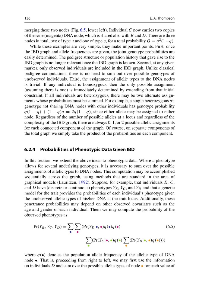
Pr(Y E , Y C , Y D ) =
•
•
(Pr(Y E |•, •)q(•)q(•)
(6.5)
•
(Pr(Y C |•, •)q(•)
•
(Pr(Y D |•, •)q(•))))
where q(•) denotes the population allele frequency of the allelic type of DNA
node •. That is, proceeding from right to left, we may first use the information
on individuals D and sum over the possible allelic types of node • for each value of
E. A. Thompson
merging these two nodes (Fig. 6.5, lower left). Individual C now carries two copies
of the sane (magenta) DNA node, which is shared also with E and D. There are three
nodes in total, two of type u and one of type v, for a total probability Q = q 2 (1−q).
While these examples are very simple, they make important points. First, once
the IBD graph and allele frequencies are given, the joint genotype probabilities are
easily determined. The pedigree structure or population history that gave rise to the
IBD graph is no longer relevant once the IBD graph is known. Second, at any given
marker, only observed individuals are included in the IBD graph. Unlike classical
pedigree computations, there is no need to sum out over possible genotypes of
unobserved individuals. Third, the assignment of allelic types to the DNA nodes
is trivial. If any individual is homozygous, then the only possible assignment
(assuming there is one) is immediately determined by extending from that initial
constraint. If all individuals are heterozygous, there may be two alternate assignments whose probabilities must be summed. For example, a single heterozygous uv
genotype not sharing DNA nodes with other individuals has genotype probability
q(1 − q) + (1 − q)q = 2q(1 − q), since either allele may be assigned to either
node. Regardless of the number of possible alleles at a locus and regardless of the
complexity of the IBD graph, there are always 0, 1, or 2 possible allelic assignments
for each connected component of the graph. Of course, on separate components of
the total graph we simply take the product of the probabilities on each component.
6.2.4 Probabilities of Phenotypic Data Given IBD
In this section, we extend the above ideas to phenotypic data. Where a phenotype
allows for several underlying genotypes, it is necessary to sum over the possible
assignments of allelic types to DNA nodes. This computation may be accomplished
sequentially across the graph, using methods that are standard in the area of
graphical models (Lauritzen, 1992). Suppose, for example, that individuals E, C,
and D have (discrete or continuous) phenotypes Y E , Y C , and Y D and that a genetic
model for the trait provides the probabilities of each individual’s phenotype given
the unobserved allelic types of his/her DNA at the trait locus. Additionally, these
penetrance probabilities may depend on other observed covariates such as the
age and gender of each individual. Them we may compute the probability of the
observed phenotypes as
Pr(Y E , Y C , Y D ) =
•
•
(Pr(Y E |•, •)q(•)q(•)
(6.5)
•
(Pr(Y C |•, •)q(•)
•
(Pr(Y D |•, •)q(•))))
where q(•) denotes the population allele frequency of the allelic type of DNA
node •. That is, proceeding from right to left, we may first use the information
on individuals D and sum over the possible allelic types of node • for each value of