

6 Identity by Descent in the Mapping of Genetic Traits
137
the type of node •. Then we can incorporate the data on individual C and for each
value of • sum over the possible values of •. Finally we may incorporate the data
on E and sum over the possible allelic types of the two remaining DNA nodes. By
processing the summation in this way, we can break the overall sum into smaller
feasible computations.
Although our example is of a small pedigree, this is for ease of presentation only.
Even for more much larger and more complex IBD graphs, these computations are
generally feasible. Where IBD graph components are small, probabilities can be
computed even under models for which the trait is controlled by genotypes at several
loci. Moreover, once the IBD graph is given, the source of that IBD information is
irrelevant. The IBD graph contains all the relevant information on the impact of
shared ancestry on joint phenotype probabilities.
A special case of phenotypic data arises with marker data where an allowance is
made for typing error. That is, the true marker genotype provides probabilities for
the marker phenotype; the observed marker “genotype” may not be the true one. In
practice, it is important to use a model that allows for the possibility of error, so that
IBD nodes are not of necessity of the same allelic type. It is not necessary to have
a model that precisely reflects biological or technological genotyping processes.
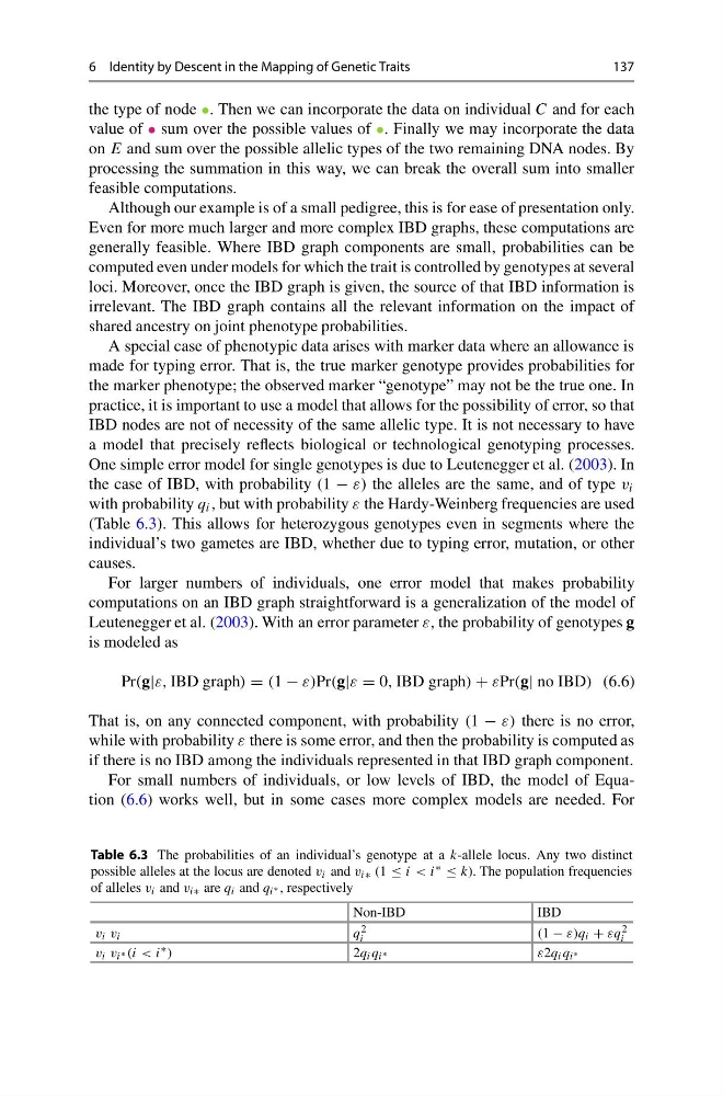
One simple error model for single genotypes is due to Leutenegger et al. (2003). In
the case of IBD, with probability (1 − ε) the alleles are the same, and of type v i
with probability q i , but with probability ε the Hardy-Weinberg frequencies are used
(Table 6.3). This allows for heterozygous genotypes even in segments where the
individual’s two gametes are IBD, whether due to typing error, mutation, or other
causes.
For larger numbers of individuals, one error model that makes probability
computations on an IBD graph straightforward is a generalization of the model of
Leutenegger et al. (2003). With an error parameter ε, the probability of genotypes g
is modeled as
Pr(g|ε, IBD graph) = (1 − ε)Pr(g|ε = 0, IBD graph) + εPr(g| no IBD) (6.6)
That is, on any connected component, with probability (1 − ε) there is no error,
while with probability ε there is some error, and then the probability is computed as
if there is no IBD among the individuals represented in that IBD graph component.
For small numbers of individuals, or low levels of IBD, the model of Equation (6.6) works well, but in some cases more complex models are needed. For
Table 6.3 The probabilities of an individual’s genotype at a k-allele locus. Any two distinct
possible alleles at the locus are denoted v i and v i∗ (1 ≤ i < i ∗ ≤ k). The population frequencies
of alleles v i and v i∗ are q i and q i ∗ , respectively
Non-IBD
IBD
v i v i
q 2
i
(1 − ε)q i + εq 2
i
v i v i ∗ (i < i ∗ )
2q i q i ∗
ε2q i q i ∗
137
the type of node •. Then we can incorporate the data on individual C and for each
value of • sum over the possible values of •. Finally we may incorporate the data
on E and sum over the possible allelic types of the two remaining DNA nodes. By
processing the summation in this way, we can break the overall sum into smaller
feasible computations.
Although our example is of a small pedigree, this is for ease of presentation only.
Even for more much larger and more complex IBD graphs, these computations are
generally feasible. Where IBD graph components are small, probabilities can be
computed even under models for which the trait is controlled by genotypes at several
loci. Moreover, once the IBD graph is given, the source of that IBD information is
irrelevant. The IBD graph contains all the relevant information on the impact of
shared ancestry on joint phenotype probabilities.
A special case of phenotypic data arises with marker data where an allowance is
made for typing error. That is, the true marker genotype provides probabilities for
the marker phenotype; the observed marker “genotype” may not be the true one. In
practice, it is important to use a model that allows for the possibility of error, so that
IBD nodes are not of necessity of the same allelic type. It is not necessary to have
a model that precisely reflects biological or technological genotyping processes.
One simple error model for single genotypes is due to Leutenegger et al. (2003). In
the case of IBD, with probability (1 − ε) the alleles are the same, and of type v i
with probability q i , but with probability ε the Hardy-Weinberg frequencies are used
(Table 6.3). This allows for heterozygous genotypes even in segments where the
individual’s two gametes are IBD, whether due to typing error, mutation, or other
causes.
For larger numbers of individuals, one error model that makes probability
computations on an IBD graph straightforward is a generalization of the model of
Leutenegger et al. (2003). With an error parameter ε, the probability of genotypes g
is modeled as
Pr(g|ε, IBD graph) = (1 − ε)Pr(g|ε = 0, IBD graph) + εPr(g| no IBD) (6.6)
That is, on any connected component, with probability (1 − ε) there is no error,
while with probability ε there is some error, and then the probability is computed as
if there is no IBD among the individuals represented in that IBD graph component.
For small numbers of individuals, or low levels of IBD, the model of Equation (6.6) works well, but in some cases more complex models are needed. For
Table 6.3 The probabilities of an individual’s genotype at a k-allele locus. Any two distinct
possible alleles at the locus are denoted v i and v i∗ (1 ≤ i < i ∗ ≤ k). The population frequencies
of alleles v i and v i∗ are q i and q i ∗ , respectively
Non-IBD
IBD
v i v i
q 2
i
(1 − ε)q i + εq 2
i
v i v i ∗ (i < i ∗ )
2q i q i ∗
ε2q i q i ∗