

354
equilibrium) genotypic proportions (average Fis = 0.021) nor a significant genotyping linkage disequilibrium (P > 0.05). Sixty-two alleles were detected in the 107
individuals analyzed through SSR markers. Allelic multiplicity showed an average
of 8.85 alleles per locus (SD = 4.09) and ranged from 5 to 16 alleles. Also, a total of
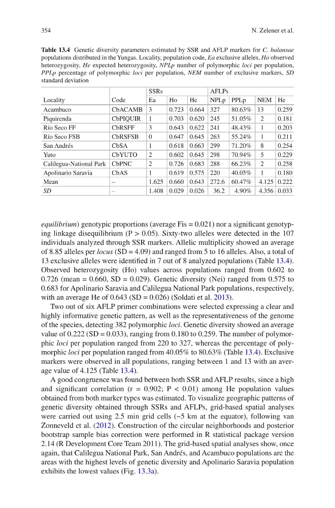
13 exclusive alleles were identified in 7 out of 8 analyzed populations (Table 13.4).
Observed heterozygosity (Ho) values across populations ranged from 0.602 to
0.726 (mean = 0.660, SD = 0.029). Genetic diversity (Nei) ranged from 0.575 to
0.683 for Apolinario Saravia and Calilegua National Park populations, respectively,
with an average He of 0.643 (SD = 0.026) (Soldati et al. 2013).
Two out of six AFLP primer combinations were selected expressing a clear and
highly informative genetic pattern, as well as the representativeness of the genome
of the species, detecting 382 polymorphic loci. Genetic diversity showed an average
value of 0.222 (SD = 0.033), ranging from 0.180 to 0.259. The number of polymorphic loci per population ranged from 220 to 327, whereas the percentage of polymorphic loci per population ranged from 40.05% to 80.63% (Table 13.4). Exclusive
markers were observed in all populations, ranging between 1 and 13 with an average value of 4.125 (Table 13.4).
A good congruence was found between both SSR and AFLP results, since a high
and significant correlation (r = 0.902; P < 0.01) among He population values
obtained from both marker types was estimated. To visualize geographic patterns of
genetic diversity obtained through SSRs and AFLPs, grid-based spatial analyses
were carried out using 2.5 min grid cells (~5 km at the equator), following van
Zonneveld et al. (2012). Construction of the circular neighborhoods and posterior
bootstrap sample bias correction were performed in R statistical package version
2.14 (R Development Core Team 2011). The grid-based spatial analyses show, once
again, that Calilegua National Park, San Andrés, and Acambuco populations are the
areas with the highest levels of genetic diversity and Apolinario Saravia population
exhibits the lowest values (Fig. 13.3a).
Table 13.4 Genetic diversity parameters estimated by SSR and AFLP markers for C. balansae
populations distributed in the Yungas. Locality, population code, Ea exclusive alleles, Ho observed
heterozygosity, He expected heterozygosity, NPLp number of polymorphic loci per population,
PPLp percentage of polymorphic loci per population, NEM number of exclusive markers, SD
standard deviation
Locality
Code
SSRs
AFLPs
Ea
Ho
He
NPLp PPLp
NEM He
Acambuco
CbACAMB 3
0.723 0.664 327
80.63% 13
0.259
Piquirenda
CbPIQUIR 1
0.703 0.620 245
51.05% 2
0.181
Río Seco FF
CbRSFF
3
0.643 0.622 241
48.43% 1
0.203
Río Seco FSB
CbRSFSB
0
0.647 0.645 263
55.24% 1
0.211
San Andrés
CbSA
1
0.618 0.663 299
71.20% 8
0.254
Yuto
CbYUTO
2
0.602 0.645 298
70.94% 5
0.229
Calilegua-National Park CbPNC
2
0.726 0.683 288
66.23% 2
0.258
Apolinario Saravia
CbAS
1
0.619 0.575 220
40.05% 1
0.180
Mean
–
1.625 0.660 0.643 272.6 60.47% 4.125 0.222
SD
–
1.408 0.029 0.026 36.2
4.90% 4.356 0.033
N. Zelener et al.
equilibrium) genotypic proportions (average Fis = 0.021) nor a significant genotyping linkage disequilibrium (P > 0.05). Sixty-two alleles were detected in the 107
individuals analyzed through SSR markers. Allelic multiplicity showed an average
of 8.85 alleles per locus (SD = 4.09) and ranged from 5 to 16 alleles. Also, a total of
13 exclusive alleles were identified in 7 out of 8 analyzed populations (Table 13.4).
Observed heterozygosity (Ho) values across populations ranged from 0.602 to
0.726 (mean = 0.660, SD = 0.029). Genetic diversity (Nei) ranged from 0.575 to
0.683 for Apolinario Saravia and Calilegua National Park populations, respectively,
with an average He of 0.643 (SD = 0.026) (Soldati et al. 2013).
Two out of six AFLP primer combinations were selected expressing a clear and
highly informative genetic pattern, as well as the representativeness of the genome
of the species, detecting 382 polymorphic loci. Genetic diversity showed an average
value of 0.222 (SD = 0.033), ranging from 0.180 to 0.259. The number of polymorphic loci per population ranged from 220 to 327, whereas the percentage of polymorphic loci per population ranged from 40.05% to 80.63% (Table 13.4). Exclusive
markers were observed in all populations, ranging between 1 and 13 with an average value of 4.125 (Table 13.4).
A good congruence was found between both SSR and AFLP results, since a high
and significant correlation (r = 0.902; P < 0.01) among He population values
obtained from both marker types was estimated. To visualize geographic patterns of
genetic diversity obtained through SSRs and AFLPs, grid-based spatial analyses
were carried out using 2.5 min grid cells (~5 km at the equator), following van
Zonneveld et al. (2012). Construction of the circular neighborhoods and posterior
bootstrap sample bias correction were performed in R statistical package version
2.14 (R Development Core Team 2011). The grid-based spatial analyses show, once
again, that Calilegua National Park, San Andrés, and Acambuco populations are the
areas with the highest levels of genetic diversity and Apolinario Saravia population
exhibits the lowest values (Fig. 13.3a).
Table 13.4 Genetic diversity parameters estimated by SSR and AFLP markers for C. balansae
populations distributed in the Yungas. Locality, population code, Ea exclusive alleles, Ho observed
heterozygosity, He expected heterozygosity, NPLp number of polymorphic loci per population,
PPLp percentage of polymorphic loci per population, NEM number of exclusive markers, SD
standard deviation
Locality
Code
SSRs
AFLPs
Ea
Ho
He
NPLp PPLp
NEM He
Acambuco
CbACAMB 3
0.723 0.664 327
80.63% 13
0.259
Piquirenda
CbPIQUIR 1
0.703 0.620 245
51.05% 2
0.181
Río Seco FF
CbRSFF
3
0.643 0.622 241
48.43% 1
0.203
Río Seco FSB
CbRSFSB
0
0.647 0.645 263
55.24% 1
0.211
San Andrés
CbSA
1
0.618 0.663 299
71.20% 8
0.254
Yuto
CbYUTO
2
0.602 0.645 298
70.94% 5
0.229
Calilegua-National Park CbPNC
2
0.726 0.683 288
66.23% 2
0.258
Apolinario Saravia
CbAS
1
0.619 0.575 220
40.05% 1
0.180
Mean
–
1.625 0.660 0.643 272.6 60.47% 4.125 0.222
SD
–
1.408 0.029 0.026 36.2
4.90% 4.356 0.033
N. Zelener et al.