

search of error space (an “error-surface projection” [8, 11])
and are more accurate than the results of most fitting programs
(see Note 26). If 95% confidence intervals are desired, one can
select “0.95” from the “Confidence Level” section of the
“Confidence Intervals” menu followed by another fitting
session.
5. If desired, examine the results of the error-surface projection
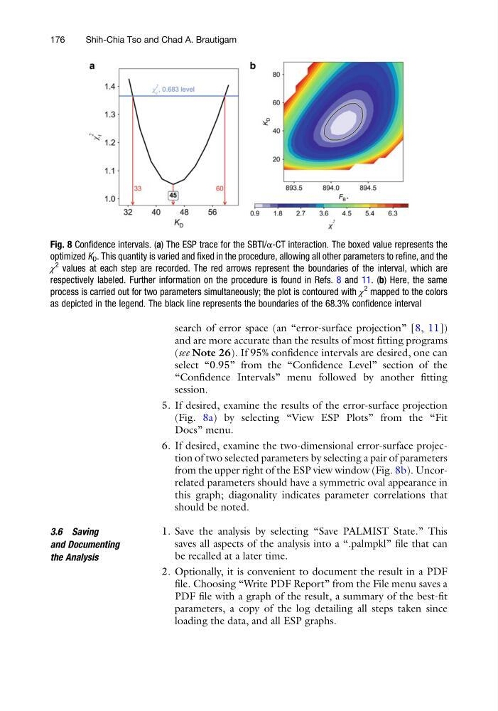
(Fig. 8a) by selecting “View ESP Plots” from the “Fit
Docs” menu.
6. If desired, examine the two-dimensional error-surface projection of two selected parameters by selecting a pair of parameters
from the upper right of the ESP view window (Fig. 8b). Uncorrelated parameters should have a symmetric oval appearance in
this graph; diagonality indicates parameter correlations that
should be noted.
3.6 Saving
and Documenting
the Analysis
1. Save the analysis by selecting “Save PALMIST State.” This
saves all aspects of the analysis into a “.palmpkl” file that can
be recalled at a later time.
2. Optionally, it is convenient to document the result in a PDF
file. Choosing “Write PDF Report” from the File menu saves a
PDF file with a graph of the result, a summary of the best-fit
parameters, a copy of the log detailing all steps taken since
loading the data, and all ESP graphs.
Fig. 8 Confidence intervals. (a) The ESP trace for the SBTI/α-CT interaction. The boxed value represents the
optimized K D . This quantity is varied and fixed in the procedure, allowing all other parameters to refine, and the
χ
2
values at each step are recorded. The red arrows represent the boundaries of the interval, which are
respectively labeled. Further information on the procedure is found in Refs. 8 and 11. (b) Here, the same
process is carried out for two parameters simultaneously; the plot is contoured with χ
2
mapped to the colors
as depicted in the legend. The black line represents the boundaries of the 68.3% confidence interval
176
Shih-Chia Tso and Chad A. Brautigam
and are more accurate than the results of most fitting programs
(see Note 26). If 95% confidence intervals are desired, one can
select “0.95” from the “Confidence Level” section of the
“Confidence Intervals” menu followed by another fitting
session.
5. If desired, examine the results of the error-surface projection
(Fig. 8a) by selecting “View ESP Plots” from the “Fit
Docs” menu.
6. If desired, examine the two-dimensional error-surface projection of two selected parameters by selecting a pair of parameters
from the upper right of the ESP view window (Fig. 8b). Uncorrelated parameters should have a symmetric oval appearance in
this graph; diagonality indicates parameter correlations that
should be noted.
3.6 Saving
and Documenting
the Analysis
1. Save the analysis by selecting “Save PALMIST State.” This
saves all aspects of the analysis into a “.palmpkl” file that can
be recalled at a later time.
2. Optionally, it is convenient to document the result in a PDF
file. Choosing “Write PDF Report” from the File menu saves a
PDF file with a graph of the result, a summary of the best-fit
parameters, a copy of the log detailing all steps taken since
loading the data, and all ESP graphs.
Fig. 8 Confidence intervals. (a) The ESP trace for the SBTI/α-CT interaction. The boxed value represents the
optimized K D . This quantity is varied and fixed in the procedure, allowing all other parameters to refine, and the
χ
2
values at each step are recorded. The red arrows represent the boundaries of the interval, which are
respectively labeled. Further information on the procedure is found in Refs. 8 and 11. (b) Here, the same
process is carried out for two parameters simultaneously; the plot is contoured with χ
2
mapped to the colors
as depicted in the legend. The black line represents the boundaries of the 68.3% confidence interval
176
Shih-Chia Tso and Chad A. Brautigam