

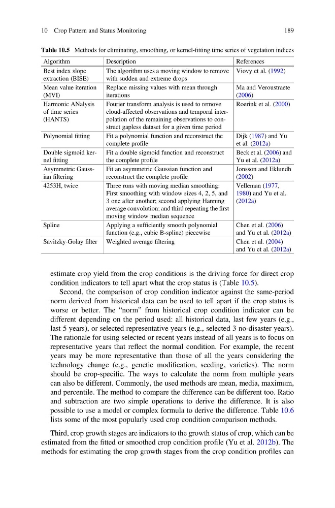
estimate crop yield from the crop conditions is the driving force for direct crop
condition indicators to tell apart what the crop status is (Table 10.5).
Second, the comparison of crop condition indicator against the same-period
norm derived from historical data can be used to tell apart if the crop status is
worse or better. The “norm” from historical crop condition indicator can be
different depending on the period used: all historical data, last few years (e.g.,
last 5 years), or selected representative years (e.g., selected 3 no-disaster years).
The rationale for using selected or recent years instead of all years is to focus on
representative years that reflect the normal condition. For example, the recent
years may be more representative than those of all the years considering the
technology change (e.g., genetic modification, seeding, varieties). The norm
should be crop-specific. The ways to calculate the norm from multiple years
can also be different. Commonly, the used methods are mean, media, maximum,
and percentile. The method to compare the difference can be different too. Ratio
and subtraction are two simple operations to derive the difference. It is also
possible to use a model or complex formula to derive the difference. Table 10.6
lists some of the most popularly used crop condition comparison methods.
Third, crop growth stages are indicators to the growth status of crop, which can be
estimated from the fitted or smoothed crop condition profile (Yu et al. 2012b). The
methods for estimating the crop growth stages from the crop condition profiles can
Table 10.5 Methods for eliminating, smoothing, or kernel-fitting time series of vegetation indices
Algorithm
Description
References
Best index slope
extraction (BISE)
The algorithm uses a moving window to remove
with sudden and extreme drops
Viovy et al. (1992)
Mean value iteration
(MVI)
Replace missing values with mean through
iterations
Ma and Veroustraete
(2006)
Harmonic ANalysis
of time series
(HANTS)
Fourier transform analysis is used to remove
cloud-affected observations and temporal interpolation of the remaining observations to construct gapless dataset for a given time period
Roerink et al. (2000)
Polynomial fitting
Fit a polynomial function and reconstruct the
complete profile
Dijk (1987) and Yu
et al. (2012a)
Double sigmoid kernel fitting
Fit a double sigmoid function and reconstruct
the complete profile
Beck et al. (2006) and
Yu et al. (2012a)
Asymmetric Gaussian filtering
Fit an asymmetric Gaussian function and
reconstruct the complete profile
Jonsson and Eklundh
(2002)
4253H, twice
Three runs with moving median smoothing:
First smoothing with window sizes 4, 2, 5, and
3 one after another; second applying Hanning
average convolution; and third repeating the first
moving window median sequence
Velleman (1977,
1980) and Yu et al.
(2012a)
Spline
Applying a sufficiently smooth polynomial
function (e.g., cubic B-spline) piecewise
Chen et al. (2006)
and Yu et al. (2012a)
Savitzky-Golay filter Weighted average filtering
Chen et al. (2004)
and Yu et al. (2012a)
10 Crop Pattern and Status Monitoring
189
condition indicators to tell apart what the crop status is (Table 10.5).
Second, the comparison of crop condition indicator against the same-period
norm derived from historical data can be used to tell apart if the crop status is
worse or better. The “norm” from historical crop condition indicator can be
different depending on the period used: all historical data, last few years (e.g.,
last 5 years), or selected representative years (e.g., selected 3 no-disaster years).
The rationale for using selected or recent years instead of all years is to focus on
representative years that reflect the normal condition. For example, the recent
years may be more representative than those of all the years considering the
technology change (e.g., genetic modification, seeding, varieties). The norm
should be crop-specific. The ways to calculate the norm from multiple years
can also be different. Commonly, the used methods are mean, media, maximum,
and percentile. The method to compare the difference can be different too. Ratio
and subtraction are two simple operations to derive the difference. It is also
possible to use a model or complex formula to derive the difference. Table 10.6
lists some of the most popularly used crop condition comparison methods.
Third, crop growth stages are indicators to the growth status of crop, which can be
estimated from the fitted or smoothed crop condition profile (Yu et al. 2012b). The
methods for estimating the crop growth stages from the crop condition profiles can
Table 10.5 Methods for eliminating, smoothing, or kernel-fitting time series of vegetation indices
Algorithm
Description
References
Best index slope
extraction (BISE)
The algorithm uses a moving window to remove
with sudden and extreme drops
Viovy et al. (1992)
Mean value iteration
(MVI)
Replace missing values with mean through
iterations
Ma and Veroustraete
(2006)
Harmonic ANalysis
of time series
(HANTS)
Fourier transform analysis is used to remove
cloud-affected observations and temporal interpolation of the remaining observations to construct gapless dataset for a given time period
Roerink et al. (2000)
Polynomial fitting
Fit a polynomial function and reconstruct the
complete profile
Dijk (1987) and Yu
et al. (2012a)
Double sigmoid kernel fitting
Fit a double sigmoid function and reconstruct
the complete profile
Beck et al. (2006) and
Yu et al. (2012a)
Asymmetric Gaussian filtering
Fit an asymmetric Gaussian function and
reconstruct the complete profile
Jonsson and Eklundh
(2002)
4253H, twice
Three runs with moving median smoothing:
First smoothing with window sizes 4, 2, 5, and
3 one after another; second applying Hanning
average convolution; and third repeating the first
moving window median sequence
Velleman (1977,
1980) and Yu et al.
(2012a)
Spline
Applying a sufficiently smooth polynomial
function (e.g., cubic B-spline) piecewise
Chen et al. (2006)
and Yu et al. (2012a)
Savitzky-Golay filter Weighted average filtering
Chen et al. (2004)
and Yu et al. (2012a)
10 Crop Pattern and Status Monitoring
189