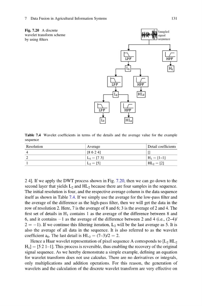
2 4]. If we apply the DWT process shown in Fig. 7.20, then we can go down to the
second layer that yields L 2 and HL 2 because there are four samples in the sequence.
The initial resolution is four, and the respective average column is the data sequence
itself as shown in Table 7.4. If we simply use the average for the low-pass filter and
the average of the difference as the high-pass filter, then we will get the data in the
row of resolution 2. Here, 7 is the average of 8 and 6; 3 is the average of 2 and 4. The
first set of details in H 1 contains 1 as the average of the difference between 8 and
6, and it contains À1 as the average of the difference between 2 and 4 (i.e., (2–4)/
2 ¼ À1). If we continue this filtering iteration, L 2 will be the last average as 5. It is
also the average of all data in the sequence. It is also referred to as the wavelet
coefficient a 0 . The last detail is HL 2 ¼ (7–3)/2 ¼ 2.
Hence a Haar wavelet representation of pixel sequence A corresponds to [L 2 HL 2
H 1 ] ¼ [5 2 1–1]. This process is reversible, thus enabling the recovery of the original
signal sequence. As we hereby demonstrate a simple example, defining an equation
for wavelet transform does not use calculus. There are no derivatives or integrals,
only multiplications and addition operations. For this reason, the generation of
wavelets and the calculation of the discrete wavelet transform are very effective on
Fig. 7.20 A discrete
wavelet transform scheme
by using filters
Table 7.4 Wavelet coefficients in terms of the details and the average value for the example
sequence
Resolution
Average
Detail coefficients
4
[ 8 6 2 4 ]
[ ]
2
L 1 ¼ [7 3]
H 1 ¼ [1–1]
1
L 2 ¼ [5]
HL 2 ¼ [2]
7 Data Fusion in Agricultural Information Systems
131