

transformation (DWT) depends on a similar convolution in discrete time. DWT
coefficients W( j, k) can be given as
W j, k
ð Þ ¼
X NÀ1
n¼0
f n
ð Þ Ã ψ
Ã
j,k n
ð Þ
ð7:22Þ
where f(n) is a sequence with length N and ψ
Ã
j,k n
ð Þ is the discretized mother wavelet
function. The superscript * denotes a complex conjugate (Smith et al. 1998). Haar
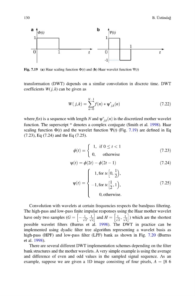
scaling function Φ(t) and the wavelet function Ψ(t) (Fig. 7.19) are defined in Eq
(7.23), Eq (7.24) and the Eq (7.25).
ϕ t
ð Þ ¼
1, if 0 t < 1
0,
otherwise
(
ð7:23Þ
ψ t
ð Þ ¼ ϕ 2t
ð Þ À ϕ 2t À 1
ð
Þ
ð7:24Þ
ψ t
ð Þ ¼
1, for tE 0,
1
2
h
,
À1, for tE
1
2
, 1
h
,
0, otherwise:
8
> > > > > <
> > > > > :
ð7:25Þ
Convolution with wavelets at certain frequencies respects the bandpass filtering.
The high-pass and low-pass finite impulse responses using the Haar mother wavelet
have only two samples (G ¼ À
1 ffiffi
2
p ,
1 ffiffi
2
p
h
i
and H ¼
1 ffiffi
2
p ,
1 ffiffi
2
p
h
i
) which are the shortest
possible wavelet filters (Burrus et al. 1998). The DWT in practice can be
implemented using dyadic filter tree algorithm representing a wavelet basis as
high-pass (HPF) and low-pass filter (LPF) bank as shown in Fig. 7.20 (Burrus
et al. 1998).
There are several different DWT implementation schemes depending on the filter
bank structures and the mother wavelets. A very simple example is using the average
and difference of even and odd values in the sampled signal sequence. As an
example, suppose we are given a 1D image consisting of four pixels, A ¼ [8 6
Fig. 7.19 (a) Haar scaling function Φ(t) and (b) Haar wavelet function Ψ(t)
130
B. Üstündağ
coefficients W( j, k) can be given as
W j, k
ð Þ ¼
X NÀ1
n¼0
f n
ð Þ Ã ψ
Ã
j,k n
ð Þ
ð7:22Þ
where f(n) is a sequence with length N and ψ
Ã
j,k n
ð Þ is the discretized mother wavelet
function. The superscript * denotes a complex conjugate (Smith et al. 1998). Haar
scaling function Φ(t) and the wavelet function Ψ(t) (Fig. 7.19) are defined in Eq
(7.23), Eq (7.24) and the Eq (7.25).
ϕ t
ð Þ ¼
1, if 0 t < 1
0,
otherwise
(
ð7:23Þ
ψ t
ð Þ ¼ ϕ 2t
ð Þ À ϕ 2t À 1
ð
Þ
ð7:24Þ
ψ t
ð Þ ¼
1, for tE 0,
1
2
h
,
À1, for tE
1
2
, 1
h
,
0, otherwise:
8
> > > > > <
> > > > > :
ð7:25Þ
Convolution with wavelets at certain frequencies respects the bandpass filtering.
The high-pass and low-pass finite impulse responses using the Haar mother wavelet
have only two samples (G ¼ À
1 ffiffi
2
p ,
1 ffiffi
2
p
h
i
and H ¼
1 ffiffi
2
p ,
1 ffiffi
2
p
h
i
) which are the shortest
possible wavelet filters (Burrus et al. 1998). The DWT in practice can be
implemented using dyadic filter tree algorithm representing a wavelet basis as
high-pass (HPF) and low-pass filter (LPF) bank as shown in Fig. 7.20 (Burrus
et al. 1998).
There are several different DWT implementation schemes depending on the filter
bank structures and the mother wavelets. A very simple example is using the average
and difference of even and odd values in the sampled signal sequence. As an
example, suppose we are given a 1D image consisting of four pixels, A ¼ [8 6
Fig. 7.19 (a) Haar scaling function Φ(t) and (b) Haar wavelet function Ψ(t)
130
B. Üstündağ