

44
Pesticides, Organic Contaminants, and Pathogens in Air
fate processes, including chemical/photochemical or microbial degradation.
Such a distribution is similar to what is observed for chemical contaminants
in a laboratory microcosm consisting of sand/soil, plants, water, and animals
(see Chapter 5).
3.4.1 Soil
3.4.1.1 Distribution between Soil/Sediment and Water
It is important to be able to measure the sorption equilibrium for a chemical
contaminant between water and soil/sediment. However, competing with
this process is the possible loss of contaminant from water to the air. This is
determined by the contaminant’s air–water partition coeffcient (K aw ), which
can be expressed as
K = C /C = H/RT
a
(3.23)
aw
w
where C a is concentration in air, C w is concentration in water, H (Pa·m 3 /mol)
is the Henry’s law coeffcient, and R is the gas constant (8.314 Pa·m 3 /mol K).
The sorption equilibrium for a contaminant between water and soil can be
illustrated as follows:
(
) + solute free
( )
Kf Solid-solute bound or sorbed)
Solid adsorbent
˛
(
(3.24)
Typically this is done by preparing multiple replicates of adsorbent (e.g.,
soil) in an Erlenmeyer fask or other suitable container, then adding six or
more different initial concentrations of solute in water, containing a known
concentration of solute stated as µg/mL. The mixtures are then shaken for
several hours to establish equilibration between water and soil, then fltered
or decanted to yield the aqueous supernatant. The concentration of solute
is then measured as C (µg/mL) in water, and concentration in soil as x/m
in µg/g. Soil concentration (x/m) is then plotted vs. C (water concentration).
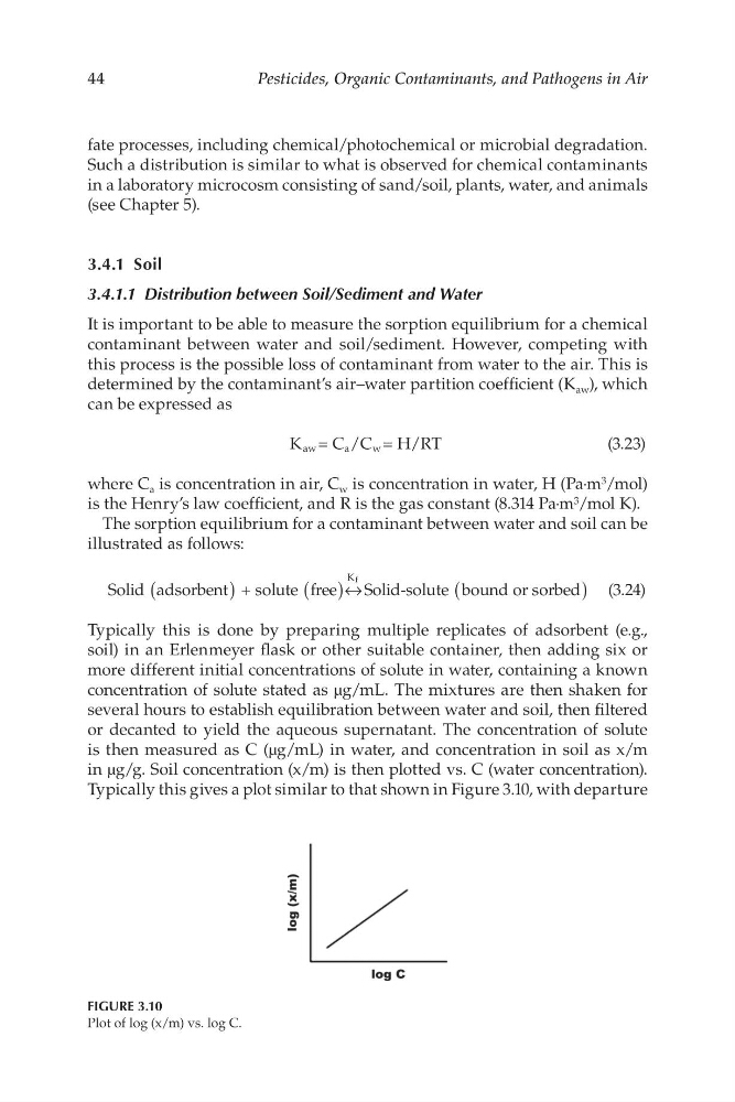
Typically this gives a plot similar to that shown in Figure 3.10, with departure
FIGURE 3.10
Plot of log (x/m) vs. log C.
Pesticides, Organic Contaminants, and Pathogens in Air
fate processes, including chemical/photochemical or microbial degradation.
Such a distribution is similar to what is observed for chemical contaminants
in a laboratory microcosm consisting of sand/soil, plants, water, and animals
(see Chapter 5).
3.4.1 Soil
3.4.1.1 Distribution between Soil/Sediment and Water
It is important to be able to measure the sorption equilibrium for a chemical
contaminant between water and soil/sediment. However, competing with
this process is the possible loss of contaminant from water to the air. This is
determined by the contaminant’s air–water partition coeffcient (K aw ), which
can be expressed as
K = C /C = H/RT
a
(3.23)
aw
w
where C a is concentration in air, C w is concentration in water, H (Pa·m 3 /mol)
is the Henry’s law coeffcient, and R is the gas constant (8.314 Pa·m 3 /mol K).
The sorption equilibrium for a contaminant between water and soil can be
illustrated as follows:
(
) + solute free
( )
Kf Solid-solute bound or sorbed)
Solid adsorbent
˛
(
(3.24)
Typically this is done by preparing multiple replicates of adsorbent (e.g.,
soil) in an Erlenmeyer fask or other suitable container, then adding six or
more different initial concentrations of solute in water, containing a known
concentration of solute stated as µg/mL. The mixtures are then shaken for
several hours to establish equilibration between water and soil, then fltered
or decanted to yield the aqueous supernatant. The concentration of solute
is then measured as C (µg/mL) in water, and concentration in soil as x/m
in µg/g. Soil concentration (x/m) is then plotted vs. C (water concentration).
Typically this gives a plot similar to that shown in Figure 3.10, with departure
FIGURE 3.10
Plot of log (x/m) vs. log C.