

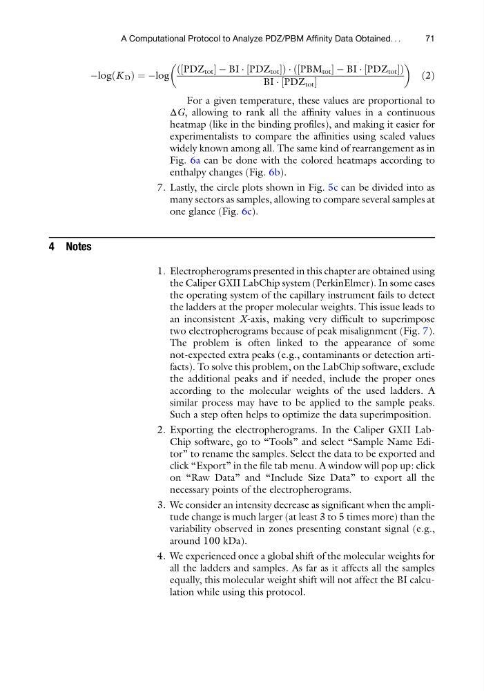
ÀlogðK D Þ ¼ Àlog
ð½PDZ tot À BI Á ½PDZ tot Þ Á ð½PBM tot À BI Á ½PDZ tot Þ
BI Á ½PDZ tot
ð2Þ
For a given temperature, these values are proportional to
ΔG, allowing to rank all the affinity values in a continuous
heatmap (like in the binding profiles), and making it easier for
experimentalists to compare the affinities using scaled values
widely known among all. The same kind of rearrangement as in
Fig. 6a can be done with the colored heatmaps according to
enthalpy changes (Fig. 6b).
7. Lastly, the circle plots shown in Fig. 5c can be divided into as
many sectors as samples, allowing to compare several samples at
one glance (Fig. 6c).
4 Notes
1. Electropherograms presented in this chapter are obtained using
the Caliper GXII LabChip system (PerkinElmer). In some cases
the operating system of the capillary instrument fails to detect
the ladders at the proper molecular weights. This issue leads to
an inconsistent X-axis, making very difficult to superimpose
two electropherograms because of peak misalignment (Fig. 7).
The problem is often linked to the appearance of some
not-expected extra peaks (e.g., contaminants or detection artifacts). To solve this problem, on the LabChip software, exclude
the additional peaks and if needed, include the proper ones
according to the molecular weights of the used ladders. A
similar process may have to be applied to the sample peaks.
Such a step often helps to optimize the data superimposition.
2. Exporting the electropherograms. In the Caliper GXII LabChip software, go to “Tools” and select “Sample Name Editor” to rename the samples. Select the data to be exported and
click “Export” in the file tab menu. A window will pop up: click
on “Raw Data” and “Include Size Data” to export all the
necessary points of the electropherograms.
3. We consider an intensity decrease as significant when the amplitude change is much larger (at least 3 to 5 times more) than the
variability observed in zones presenting constant signal (e.g.,
around 100 kDa).
4. We experienced once a global shift of the molecular weights for
all the ladders and samples. As far as it affects all the samples
equally, this molecular weight shift will not affect the BI calculation while using this protocol.
A Computational Protocol to Analyze PDZ/PBM Affinity Data Obtained. . .
71
ð½PDZ tot À BI Á ½PDZ tot Þ Á ð½PBM tot À BI Á ½PDZ tot Þ
BI Á ½PDZ tot
ð2Þ
For a given temperature, these values are proportional to
ΔG, allowing to rank all the affinity values in a continuous
heatmap (like in the binding profiles), and making it easier for
experimentalists to compare the affinities using scaled values
widely known among all. The same kind of rearrangement as in
Fig. 6a can be done with the colored heatmaps according to
enthalpy changes (Fig. 6b).
7. Lastly, the circle plots shown in Fig. 5c can be divided into as
many sectors as samples, allowing to compare several samples at
one glance (Fig. 6c).
4 Notes
1. Electropherograms presented in this chapter are obtained using
the Caliper GXII LabChip system (PerkinElmer). In some cases
the operating system of the capillary instrument fails to detect
the ladders at the proper molecular weights. This issue leads to
an inconsistent X-axis, making very difficult to superimpose
two electropherograms because of peak misalignment (Fig. 7).
The problem is often linked to the appearance of some
not-expected extra peaks (e.g., contaminants or detection artifacts). To solve this problem, on the LabChip software, exclude
the additional peaks and if needed, include the proper ones
according to the molecular weights of the used ladders. A
similar process may have to be applied to the sample peaks.
Such a step often helps to optimize the data superimposition.
2. Exporting the electropherograms. In the Caliper GXII LabChip software, go to “Tools” and select “Sample Name Editor” to rename the samples. Select the data to be exported and
click “Export” in the file tab menu. A window will pop up: click
on “Raw Data” and “Include Size Data” to export all the
necessary points of the electropherograms.
3. We consider an intensity decrease as significant when the amplitude change is much larger (at least 3 to 5 times more) than the
variability observed in zones presenting constant signal (e.g.,
around 100 kDa).
4. We experienced once a global shift of the molecular weights for
all the ladders and samples. As far as it affects all the samples
equally, this molecular weight shift will not affect the BI calculation while using this protocol.
A Computational Protocol to Analyze PDZ/PBM Affinity Data Obtained. . .
71