86 Computational Modelling in Hydraulic and Coastal Engineering
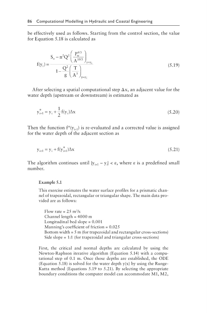
be effectively used as follows. Starting from the control section, the value
for Equation 5.18 is calculated as
f y
S n Q
P
A
Q
g
T
A
i
o
w
y y i
( )
/
/
=
−

 

 
−

 

 
=
2 2
4 3
10 3
2
3
1
y y y i
=
(5.19)
After selecting a spatial computational step Δx, an adjacent value for the
water depth (upstream or downstream) is estimated as
y
y
f y x
i
i
i
+ = +
1
1
2
*
( )∆
(5.20)
Then the function f*(y i+1 ) is re-evaluated and a corrected value is assigned
for the water depth of the adjacent section as
y
y f y
x
i
i
i
+
+
= +
1
1
( * )∆
(5.21)
The algorithm continues until ∣y i+1 – y i ∣ < ε, where ε is a predefined small
number.
Example 5.1
This exercise estimates the water surface profiles for a prismatic channel of trapezoidal, rectangular or triangular shape. The main data provided are as follows:
Flow rate = 25 m 3 /s
Channel length = 4000 m
Longitudinal bed slope = 0.001
Manning’s coefficient of friction = 0.025
Bottom width = 5 m (for trapezoidal and rectangular cross-sections)
Side slope = 1:1 (for trapezoidal and triangular cross-sections)
First, the critical and normal depths are calculated by using the
Newton-Raphson iterative algorithm (Equation 5.14) with a computational step of 0.1 m. Once those depths are established, the ODE
(Equation 5.18) is solved for the water depth y(x) by using the RungeKutta method (Equations 5.19 to 5.21). By selecting the appropriate
boundary conditions the computer model can accommodate M1, M2,