

Free surface flows 87
S2 and S3 surface profiles. More specifically, some suggested boundary
conditions are
M1 profile: Y d = 1.5y n
M2 profile: Y d = (y n + y c )/2
S2 profile: Y u = (y n + y c )/2
S3 profile: Y u = 0.1y n
where Y d and Y u are the water depths at the downstream and upstream
control section, respectively. The computational step was selected as
Δx = 1 m.
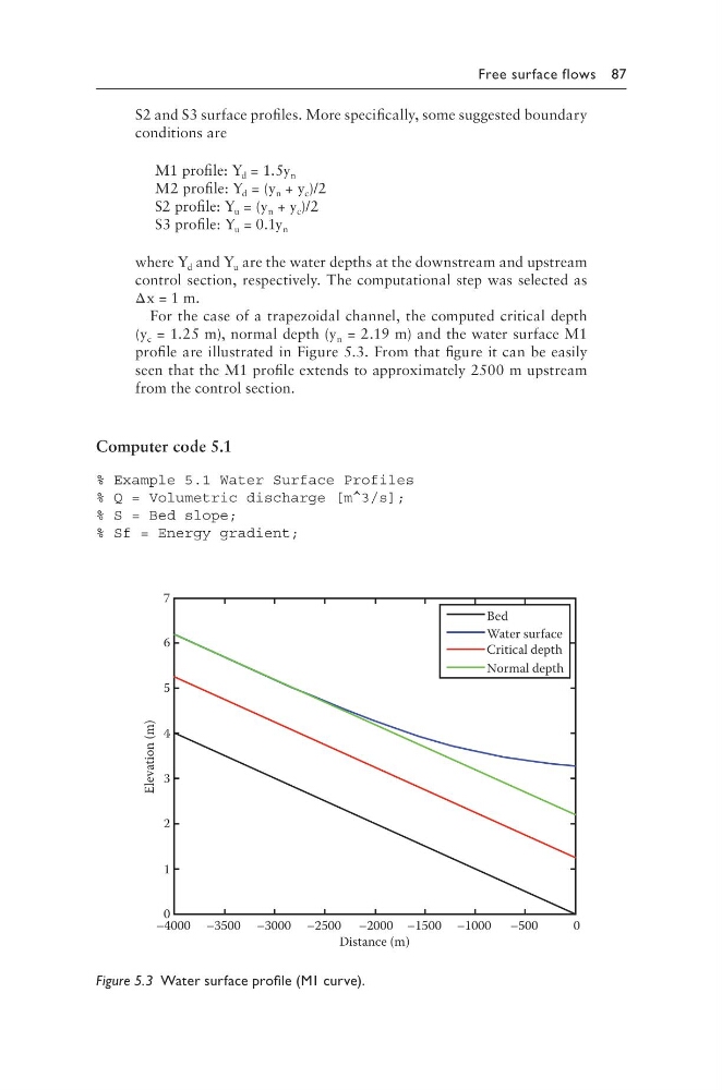
For the case of a trapezoidal channel, the computed critical depth
(y c = 1.25 m), normal depth (y n = 2.19 m) and the water surface M1
profile are illustrated in Figure 5.3. From that figure it can be easily
seen that the M1 profile extends to approximately 2500 m upstream
from the control section.
Computer code 5.1
% Example 5.1 Water Surface Profiles
% Q = Volumetric discharge [m^3/s];
% S = Bed slope;
% Sf = Energy gradient;
7
6
5
4
3
2
1
0
–4000 –3500 –3000 –2500 –2000 –1500 –1000 –500
0
Elevation (m)
Distance (m)
Bed
Water surface
Critical depth
Normal depth
Figure 5.3 Water surface profile (M1 curve).
S2 and S3 surface profiles. More specifically, some suggested boundary
conditions are
M1 profile: Y d = 1.5y n
M2 profile: Y d = (y n + y c )/2
S2 profile: Y u = (y n + y c )/2
S3 profile: Y u = 0.1y n
where Y d and Y u are the water depths at the downstream and upstream
control section, respectively. The computational step was selected as
Δx = 1 m.
For the case of a trapezoidal channel, the computed critical depth
(y c = 1.25 m), normal depth (y n = 2.19 m) and the water surface M1
profile are illustrated in Figure 5.3. From that figure it can be easily
seen that the M1 profile extends to approximately 2500 m upstream
from the control section.
Computer code 5.1
% Example 5.1 Water Surface Profiles
% Q = Volumetric discharge [m^3/s];
% S = Bed slope;
% Sf = Energy gradient;
7
6
5
4
3
2
1
0
–4000 –3500 –3000 –2500 –2000 –1500 –1000 –500
0
Elevation (m)
Distance (m)
Bed
Water surface
Critical depth
Normal depth
Figure 5.3 Water surface profile (M1 curve).