84 Computational Modelling in Hydraulic and Coastal Engineering
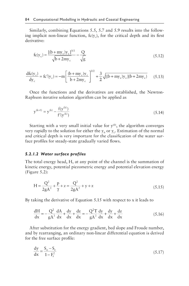
Similarly, combining Equations 5.5, 5.7 and 5.9 results into the following implicit non-linear function, fc(y c ), for the critical depth and its first
derivative:
fc y
b my y
b my
Q
g
c
c
c
c
( )
[(
) ]
/
=
+
+
−
3 2
2
(5.12)
dfc y
dy
fc y
m
b my y
b my
c
c
c
c
c
c
( )
( )
(
)
/
= ′
= −
+
+





 +
2
3
3 2
2 2
2
[(
) ](
)
b my y b
my
c
c
c
+
+
(5.13)
Once the functions and the derivatives are established, the NewtonRaphson iterative solution algorithm can be applied as
y
y
f y
f y
k
k
k
k
(
)
( )
( )
( )
( )
( )
+
=
− ′
1
(5.14)
Starting with a very small initial value for y (0) , the algorithm converges
very rapidly to the solution for either the y n or y c . Estimation of the normal
and critical depth is very important for the classification of the water surface profiles for steady-state gradually varied flows.
5.2.1.2 Water surface profiles
The total energy head, H, at any point of the channel is the summation of
kinetic energy, potential piezometric energy and potential elevation energy
(Figure 5.2):
H
Q
gA
p z
Q
gA
y z
=
+ + =
+ +
2
2
2
2
2
2
γ
(5.15)
By taking the derivative of Equation 5.15 with respect to x it leads to
dH
dx
Q
gA
dA
dx
dy
dx
dz
dx
Q T
gA
dy
dx
dy
dx
dz
dx
= −
+
+
= −
+
+
2
3
2
3
(5.16)
After substitution for the energy gradient, bed slope and Froude number,
and by rearranging, an ordinary non-linear differential equation is derived
for the free surface profile:
dy
dx
S S
F
o
e
r
=
−
−
1
2
(5.17)