

74 Computational Modelling in Hydraulic and Coastal Engineering
Example 4.2
This exercise examines the development of water hammer effects in a
pipe after the closure of a vane. The data provided are
Water height in the reservoir = 5.0 m
Elastic wave celerity = 500 m/s
Spatial cell size = 50 m
Number of cells = 100
Pipe diameter = 2 m
Wall friction coefficient (K f ) = 0.05
Valve closure time = 5 s, 20 s, 40 s
The numerical scheme used is given by Equations 4.33 and 4.34. The
time step is 0.02 seconds and the simulation ran for 10,000 time steps.
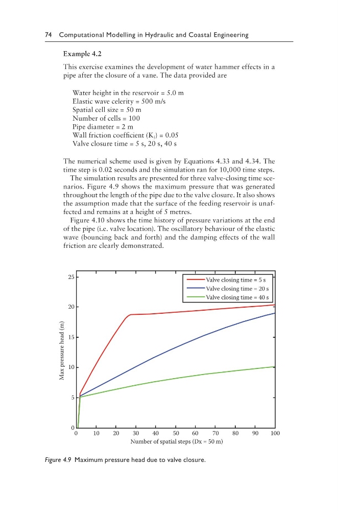
The simulation results are presented for three valve-closing time scenarios. Figure 4.9 shows the maximum pressure that was generated
throughout the length of the pipe due to the valve closure. It also shows
the assumption made that the surface of the feeding reservoir is unaffected and remains at a height of 5 metres.
Figure 4.10 shows the time history of pressure variations at the end
of the pipe (i.e. valve location). The oscillatory behaviour of the elastic
wave (bouncing back and forth) and the damping effects of the wall
friction are clearly demonstrated.
25
20
15
10
5
0 0
10
20
30
40
50
60
70
80
90
100
Number of spatial steps (Dx = 50 m)
Max pressure head (m)
Valve closing time = 5 s
Valve closing time = 20 s
Valve closing time = 40 s
Figure 4.9 Maximum pressure head due to valve closure.
Example 4.2
This exercise examines the development of water hammer effects in a
pipe after the closure of a vane. The data provided are
Water height in the reservoir = 5.0 m
Elastic wave celerity = 500 m/s
Spatial cell size = 50 m
Number of cells = 100
Pipe diameter = 2 m
Wall friction coefficient (K f ) = 0.05
Valve closure time = 5 s, 20 s, 40 s
The numerical scheme used is given by Equations 4.33 and 4.34. The
time step is 0.02 seconds and the simulation ran for 10,000 time steps.
The simulation results are presented for three valve-closing time scenarios. Figure 4.9 shows the maximum pressure that was generated
throughout the length of the pipe due to the valve closure. It also shows
the assumption made that the surface of the feeding reservoir is unaffected and remains at a height of 5 metres.
Figure 4.10 shows the time history of pressure variations at the end
of the pipe (i.e. valve location). The oscillatory behaviour of the elastic
wave (bouncing back and forth) and the damping effects of the wall
friction are clearly demonstrated.
25
20
15
10
5
0 0
10
20
30
40
50
60
70
80
90
100
Number of spatial steps (Dx = 50 m)
Max pressure head (m)
Valve closing time = 5 s
Valve closing time = 20 s
Valve closing time = 40 s
Figure 4.9 Maximum pressure head due to valve closure.