

Common partial differential equations of computational hydraulics 35
Example 3.1
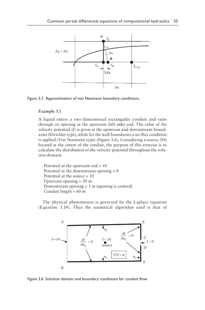
A liquid enters a two-dimensional rectangular conduit and exits
through an opening at the upstream (left side) end. The value of the
velocity potential (f) is given at the upstream and downstream boundaries (Dirichlet type), while for the wall boundaries a no-flux condition
is applied (Von Neumann type) (Figure 3.6). Considering a source (SS)
located at the centre of the conduit, the purpose of this exercise is to
calculate the distribution of the velocity potential throughout the solution domain:
Potential at the upstream end = 10
Potential at the downstream opening = 0
Potential at the source = 10
Upstream opening = 30 m
Downstream opening = 5 m (opening is centred)
Conduit length = 60 m
The physical phenomenon is governed by the Laplace equation
(Equation 3.14). Thus the numerical algorithm used is that of
f i,j
f i+1,j
Δs
λΔx
f B
f A
B
A
Δy = Δx
Δx
Figure 3.5 Approximation of von Neumann boundary conditions.
f = 10
f = 0
f = 10
source
n y
n y
n x
B
A
C
D
E
F
∆
2 f = 0
∂f
∂n y
= 0
∂f
∂n x
= 0
Figure 3.6 Solution domain and boundary conditions for conduit flow.
Example 3.1
A liquid enters a two-dimensional rectangular conduit and exits
through an opening at the upstream (left side) end. The value of the
velocity potential (f) is given at the upstream and downstream boundaries (Dirichlet type), while for the wall boundaries a no-flux condition
is applied (Von Neumann type) (Figure 3.6). Considering a source (SS)
located at the centre of the conduit, the purpose of this exercise is to
calculate the distribution of the velocity potential throughout the solution domain:
Potential at the upstream end = 10
Potential at the downstream opening = 0
Potential at the source = 10
Upstream opening = 30 m
Downstream opening = 5 m (opening is centred)
Conduit length = 60 m
The physical phenomenon is governed by the Laplace equation
(Equation 3.14). Thus the numerical algorithm used is that of
f i,j
f i+1,j
Δs
λΔx
f B
f A
B
A
Δy = Δx
Δx
Figure 3.5 Approximation of von Neumann boundary conditions.
f = 10
f = 0
f = 10
source
n y
n y
n x
B
A
C
D
E
F
∆
2 f = 0
∂f
∂n y
= 0
∂f
∂n x
= 0
Figure 3.6 Solution domain and boundary conditions for conduit flow.