

36 Computational Modelling in Hydraulic and Coastal Engineering
Equation 3.18. The computational grid is defined as 30 × 60, and the
number of iterations is set equal to 1000.
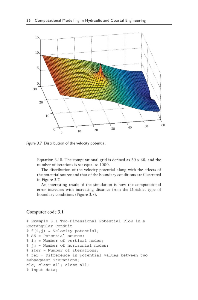
The distribution of the velocity potential along with the effects of
the potential source and that of the boundary conditions are illustrated
in Figure 3.7.
An interesting result of the simulation is how the computational
error increases with increasing distance from the Dirichlet type of
boundary conditions (Figure 3.8).
Computer code 3.1
% Example 3.1 Two-Dimensional Potential Flow in a
Rectangular Conduit
% f(i,j) = Velocity potential;
% SS = Potential source;
% im = Number of vertical nodes;
% jm = Number of horizontal nodes;
% iter = Number of iterations;
% fer = Difference in potential values between two
subsequent iterations;
clc; clear all; close all;
% Input data;
15
10
5
0
30
20
10
0 0
10
20
30
40
50
60
Figure 3.7 Distribution of the velocity potential.
Equation 3.18. The computational grid is defined as 30 × 60, and the
number of iterations is set equal to 1000.
The distribution of the velocity potential along with the effects of
the potential source and that of the boundary conditions are illustrated
in Figure 3.7.
An interesting result of the simulation is how the computational
error increases with increasing distance from the Dirichlet type of
boundary conditions (Figure 3.8).
Computer code 3.1
% Example 3.1 Two-Dimensional Potential Flow in a
Rectangular Conduit
% f(i,j) = Velocity potential;
% SS = Potential source;
% im = Number of vertical nodes;
% jm = Number of horizontal nodes;
% iter = Number of iterations;
% fer = Difference in potential values between two
subsequent iterations;
clc; clear all; close all;
% Input data;
15
10
5
0
30
20
10
0 0
10
20
30
40
50
60
Figure 3.7 Distribution of the velocity potential.