

34 Computational Modelling in Hydraulic and Coastal Engineering
3.3.1.2 Approximation of boundary conditions
The main challenge in the numerical solution of elliptic equations is the
approximation of boundary conditions involving solution points on or near
the boundaries. The computational speed of modern computers permits the
discretization of the solution domain using a small discretization step, so
the approximation of the boundaries of complex geometry does not present
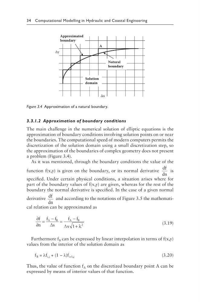
a problem (Figure 3.4).
As it was mentioned, through the boundary conditions the value of the
function f(x,y) is given on the boundary, or its normal derivative
df
dn
is
specified. Under certain physical conditions, a situation arises where for
part of the boundary values of f(x,y) are given, whereas for the rest of the
boundary the normal derivative is specified. In the case of a given normal
derivative
df
dn
and according to the notations of Figure 3.5 the mathematical relation can be approximated as
∂
∂
=
− =
−
+
f
n
f
f
s
f
f
x
A
B
A
B
∆
∆ 1
2
λ
(3.19)
Furthermore f B can be expressed by linear interpolation in terms of f(x,y)
values from the interior of the solution domain as
f B = λf i,j + (1 − λ)f i+1,j
(3.20)
Thus, the value of function f A on the discretized boundary point A can be
expressed by means of interior values of that function.
Δy
Δx
A
Natural
boundary
Approximated
boundary
Solution
domain
Figure 3.4 Approximation of a natural boundary.
3.3.1.2 Approximation of boundary conditions
The main challenge in the numerical solution of elliptic equations is the
approximation of boundary conditions involving solution points on or near
the boundaries. The computational speed of modern computers permits the
discretization of the solution domain using a small discretization step, so
the approximation of the boundaries of complex geometry does not present
a problem (Figure 3.4).
As it was mentioned, through the boundary conditions the value of the
function f(x,y) is given on the boundary, or its normal derivative
df
dn
is
specified. Under certain physical conditions, a situation arises where for
part of the boundary values of f(x,y) are given, whereas for the rest of the
boundary the normal derivative is specified. In the case of a given normal
derivative
df
dn
and according to the notations of Figure 3.5 the mathematical relation can be approximated as
∂
∂
=
− =
−
+
f
n
f
f
s
f
f
x
A
B
A
B
∆
∆ 1
2
λ
(3.19)
Furthermore f B can be expressed by linear interpolation in terms of f(x,y)
values from the interior of the solution domain as
f B = λf i,j + (1 − λ)f i+1,j
(3.20)
Thus, the value of function f A on the discretized boundary point A can be
expressed by means of interior values of that function.
Δy
Δx
A
Natural
boundary
Approximated
boundary
Solution
domain
Figure 3.4 Approximation of a natural boundary.