

Common partial differential equations of computational hydraulics 31
3.3 NUMERICAL SOLUTIONS OF TYPICAL
PARTIAL DIFFERENTIAL EQUATIONS
In the following, numerical solutions of representative PDEs and associated
hydraulic problems will be discussed. For simplicity, solutions are limited
to applications involving one or two spatial dimensions (Rezzolla 2011).
The first step for the numerical solution is the discretization of the space–
time solution domain by means of a regular grid with mesh sizes Δx, Δy
and Δt. In the case of a two-dimensional space, the grids used, without any
loss of generality, are square grids (Δx = Δy). As previously mentioned, the
numerical solution is defined as the numerical calculation of the values of
function f(x,y,t) on some pre-determined points of the discretisation grid such
as the nodes, the sides or the centres of the cells. This calculation is accomplished by discretizing the differential equation and solving the resulting
algebraic equation (explicit scheme) or system of equations (implicit scheme)
for the unknown values of the function on the grid points. Of course, due
to the fact that boundary and initial conditions must be provided, the values
of function f(x,y,t) corresponding to those conditions would be known. For
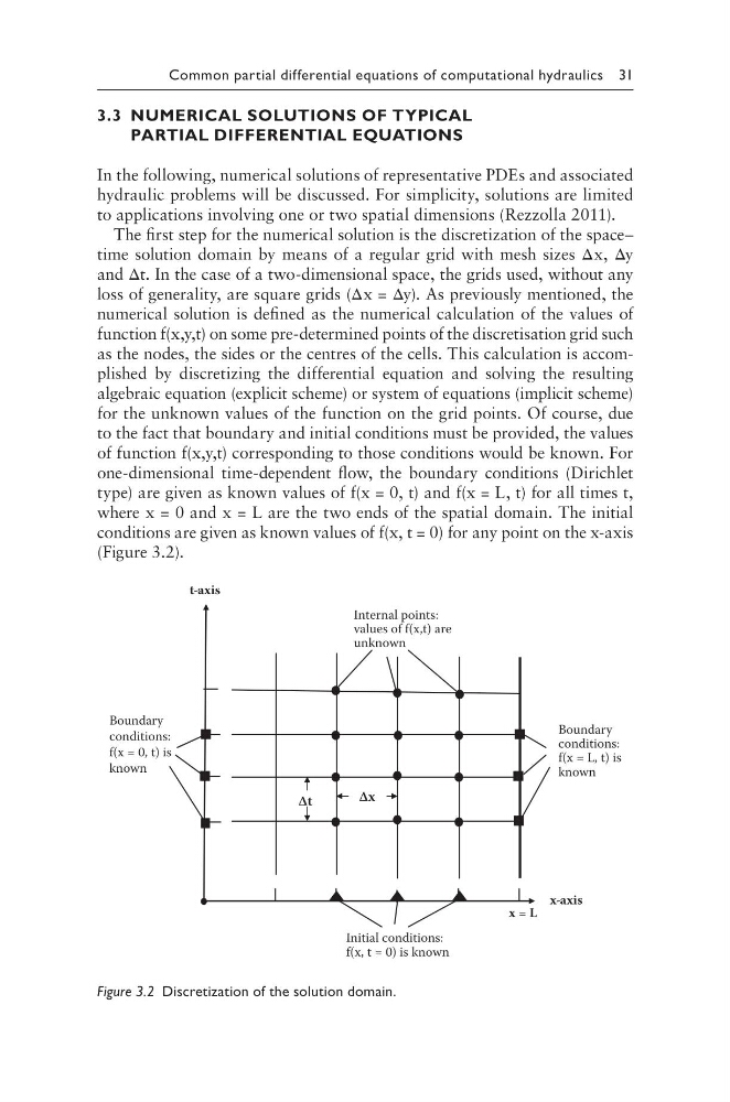
one-dimensional time-dependent flow, the boundary conditions (Dirichlet
type) are given as known values of f(x = 0, t) and f(x = L, t) for all times t,
where x = 0 and x = L are the two ends of the spatial domain. The initial
conditions are given as known values of f(x, t = 0) for any point on the x-axis
(Figure 3.2).
x = L
x-axis
Internal points:
values of f(x,t) are
unknown
t-axis
Δx
Δt
Boundary
conditions:
f(x = 0, t) is
known
Boundary
conditions:
f(x = L, t) is
known
Initial conditions:
f(x, t = 0) is known
Figure 3.2 Discretization of the solution domain.
3.3 NUMERICAL SOLUTIONS OF TYPICAL
PARTIAL DIFFERENTIAL EQUATIONS
In the following, numerical solutions of representative PDEs and associated
hydraulic problems will be discussed. For simplicity, solutions are limited
to applications involving one or two spatial dimensions (Rezzolla 2011).
The first step for the numerical solution is the discretization of the space–
time solution domain by means of a regular grid with mesh sizes Δx, Δy
and Δt. In the case of a two-dimensional space, the grids used, without any
loss of generality, are square grids (Δx = Δy). As previously mentioned, the
numerical solution is defined as the numerical calculation of the values of
function f(x,y,t) on some pre-determined points of the discretisation grid such
as the nodes, the sides or the centres of the cells. This calculation is accomplished by discretizing the differential equation and solving the resulting
algebraic equation (explicit scheme) or system of equations (implicit scheme)
for the unknown values of the function on the grid points. Of course, due
to the fact that boundary and initial conditions must be provided, the values
of function f(x,y,t) corresponding to those conditions would be known. For
one-dimensional time-dependent flow, the boundary conditions (Dirichlet
type) are given as known values of f(x = 0, t) and f(x = L, t) for all times t,
where x = 0 and x = L are the two ends of the spatial domain. The initial
conditions are given as known values of f(x, t = 0) for any point on the x-axis
(Figure 3.2).
x = L
x-axis
Internal points:
values of f(x,t) are
unknown
t-axis
Δx
Δt
Boundary
conditions:
f(x = 0, t) is
known
Boundary
conditions:
f(x = L, t) is
known
Initial conditions:
f(x, t = 0) is known
Figure 3.2 Discretization of the solution domain.