

32 Computational Modelling in Hydraulic and Coastal Engineering
3.3.1 Solution of an elliptic partial differential
equation (Laplace equation)
A two-dimensional elliptic PDE describes the distribution of a physical variable f(x,y) under equilibrium conditions. One simple expression of elliptic
equations is the Laplace equation written as
∂
∂
+
∂
∂
=
2
2
2
2
0
f
x
f
y
(3.14)
The discretization of Equation 3.14 is accomplished by approximating
the derivatives by the centred (by central) finite differences. The solution
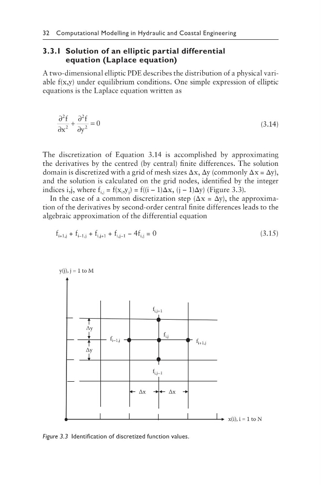
domain is discretized with a grid of mesh sizes Δx, Δy (commonly Δx = Δy),
and the solution is calculated on the grid nodes, identified by the integer
indices i,j, where f i,j = f(x i ,y j ) = f((i – 1)Δx, (j – 1)Δy) (Figure 3.3).
In the case of a common discretization step (Δx = Δy), the approximation of the derivatives by second-order central finite differences leads to the
algebraic approximation of the differential equation
f i+1,j + f i−1,j + f i,j+1 + f i,j−1 − 4f i,j = 0
(3.15)
f i,j
Δy
Δy
x(i), i = 1 to N
y(j), j = 1 to M
Δx
f i,j+1
f i,j–1
f i+1,j
Δx
f i–1,j
Figure 3.3 Identification of discretized function values.
3.3.1 Solution of an elliptic partial differential
equation (Laplace equation)
A two-dimensional elliptic PDE describes the distribution of a physical variable f(x,y) under equilibrium conditions. One simple expression of elliptic
equations is the Laplace equation written as
∂
∂
+
∂
∂
=
2
2
2
2
0
f
x
f
y
(3.14)
The discretization of Equation 3.14 is accomplished by approximating
the derivatives by the centred (by central) finite differences. The solution
domain is discretized with a grid of mesh sizes Δx, Δy (commonly Δx = Δy),
and the solution is calculated on the grid nodes, identified by the integer
indices i,j, where f i,j = f(x i ,y j ) = f((i – 1)Δx, (j – 1)Δy) (Figure 3.3).
In the case of a common discretization step (Δx = Δy), the approximation of the derivatives by second-order central finite differences leads to the
algebraic approximation of the differential equation
f i+1,j + f i−1,j + f i,j+1 + f i,j−1 − 4f i,j = 0
(3.15)
f i,j
Δy
Δy
x(i), i = 1 to N
y(j), j = 1 to M
Δx
f i,j+1
f i,j–1
f i+1,j
Δx
f i–1,j
Figure 3.3 Identification of discretized function values.