

282 Computational Modelling in Hydraulic and Coastal Engineering
Then Equation 9.117 becomes
αϕ
ϕ
ϕ
( )
( )
ln
( )
P
r
r
n
r
Q
n
ds
S
=
∂
∂
−
∂
∂
∫
Q
(9.118)
where for a smooth boundary α = π. The physical interpretation of
Equation 9.118 is the balance between potential sources (lnr) and dipoles
∂
∂
(ln )
r
n
weighted by
∂
∂
ϕ
n
and φ, respectively.
Since either φ or
∂
∂
ϕ
n
should be known, by selecting N-number of field
points Q on the boundary, an N-number of equations is generated for the
missing quantities. In summary the BEM procedure is as follows:
1. A finite number of field points Q j (j = 1,N) are defined on the boundary.
2. A different point P i (i = 1,N) is selected each time as the base point.
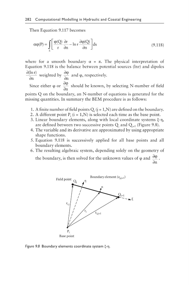
3. Linear boundary elements, along with local coordinate systems ξ-η,
are defined between two successive points Q j and Q j+1 (Figure 9.8).
4. The variable and its derivative are approximated by using appropriate
shape functions.
5. Equation 9.118 is successively applied for all base points and all
boundary elements.
6. The resulting algebraic system, depending solely on the geometry of
the boundary, is then solved for the unknown values of φ and ∂
∂
ϕ
n
.
Field point
ξ
r i,j+1
r i,j
r i
Q j+1
Boundary element (e j,j+1 )
n
Q j
η
P i
Base point
Figure 9.8 Boundary elements coordinate system ξ-η.
Then Equation 9.117 becomes
αϕ
ϕ
ϕ
( )
( )
ln
( )
P
r
r
n
r
Q
n
ds
S
=
∂
∂
−
∂
∂
∫
Q
(9.118)
where for a smooth boundary α = π. The physical interpretation of
Equation 9.118 is the balance between potential sources (lnr) and dipoles
∂
∂
(ln )
r
n
weighted by
∂
∂
ϕ
n
and φ, respectively.
Since either φ or
∂
∂
ϕ
n
should be known, by selecting N-number of field
points Q on the boundary, an N-number of equations is generated for the
missing quantities. In summary the BEM procedure is as follows:
1. A finite number of field points Q j (j = 1,N) are defined on the boundary.
2. A different point P i (i = 1,N) is selected each time as the base point.
3. Linear boundary elements, along with local coordinate systems ξ-η,
are defined between two successive points Q j and Q j+1 (Figure 9.8).
4. The variable and its derivative are approximated by using appropriate
shape functions.
5. Equation 9.118 is successively applied for all base points and all
boundary elements.
6. The resulting algebraic system, depending solely on the geometry of
the boundary, is then solved for the unknown values of φ and ∂
∂
ϕ
n
.
Field point
ξ
r i,j+1
r i,j
r i
Q j+1
Boundary element (e j,j+1 )
n
Q j
η
P i
Base point
Figure 9.8 Boundary elements coordinate system ξ-η.