

Other numerical methods 281
ϕ
ϕ
ϕ
∂
∂
−
∂
∂
+
∂
∂
−
∫
→
(ln ) ln
lim
(ln ) ln
r
n
r n
ds
r
n
S
r o 0
r r n
ds
∂
∂
=
∫
ϕ
σ
0
(9.115)
In addition, the integral around circle σ is estimated as
lim
ln
( )
r
o
o
o
o
r
r r
r d
P
→
− +
∂
∂
= −
∫
0
0
2
2
ϕ
ϕ
θ
πϕ
π
(9.116)
Combining Equations 9.115 and 9.116 results in
2πϕ
ϕ
ϕ
( )
( )
(ln ) ln
( )
P
Q
r
n
r
Q
n
ds
S
=
∂
∂
−
∂
∂
∫
(9.117)
Therefore, the potential at any interior point P of the domain D can be
estimated provided that both the potential φ and its derivative
∂
∂
ϕ
n
on
the boundary are known. In a well-posed problem, the values of either
φ (Dirichlet condition),
∂
∂
ϕ
n
(Von Neumann condition) or a combination
of both (Robin condition) are provided. But in order to apply Equation
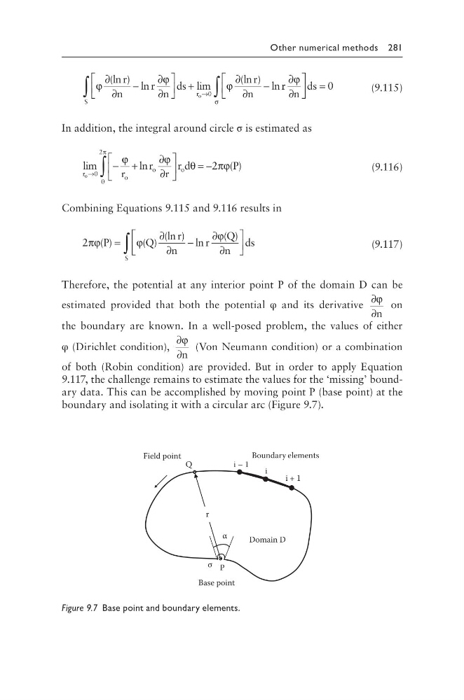
9.117, the challenge remains to estimate the values for the ‘missing’ boundary data. This can be accomplished by moving point P (base point) at the
boundary and isolating it with a circular arc (Figure 9.7).
α
σ
i
Boundary elements
i + 1
i – 1
Field point
Q
P
Domain D
r
Base point
Figure 9.7 Base point and boundary elements.
ϕ
ϕ
ϕ
∂
∂
−
∂
∂
+
∂
∂
−
∫
→
(ln ) ln
lim
(ln ) ln
r
n
r n
ds
r
n
S
r o 0
r r n
ds
∂
∂
=
∫
ϕ
σ
0
(9.115)
In addition, the integral around circle σ is estimated as
lim
ln
( )
r
o
o
o
o
r
r r
r d
P
→
− +
∂
∂
= −
∫
0
0
2
2
ϕ
ϕ
θ
πϕ
π
(9.116)
Combining Equations 9.115 and 9.116 results in
2πϕ
ϕ
ϕ
( )
( )
(ln ) ln
( )
P
Q
r
n
r
Q
n
ds
S
=
∂
∂
−
∂
∂
∫
(9.117)
Therefore, the potential at any interior point P of the domain D can be
estimated provided that both the potential φ and its derivative
∂
∂
ϕ
n
on
the boundary are known. In a well-posed problem, the values of either
φ (Dirichlet condition),
∂
∂
ϕ
n
(Von Neumann condition) or a combination
of both (Robin condition) are provided. But in order to apply Equation
9.117, the challenge remains to estimate the values for the ‘missing’ boundary data. This can be accomplished by moving point P (base point) at the
boundary and isolating it with a circular arc (Figure 9.7).
α
σ
i
Boundary elements
i + 1
i – 1
Field point
Q
P
Domain D
r
Base point
Figure 9.7 Base point and boundary elements.