

280 Computational Modelling in Hydraulic and Coastal Engineering
Furthermore, Equation 9.111 can be written as
[
]
F G G F d
F
G
n
G
F
n
ds
D
S
∇ − ∇
=
∂
∂
−
∂
∂
∫∫∫
∫∫
2
2
ω
(9.112)
In case both functions G and F satisfy the Laplace equation (∇ 2 G = ∇ 2 F =
0), then Equation 9.112 is reduced to the boundary integral
F
G
n
G
F
n
ds
S
∂
∂
−
∂
∂
=
∫∫
0
(9.113)
and the solution is simplified substantially.
9.4.2 Boundary elements method in water resources
In water resources applications it is very common to deal with velocity
potential fields. Thus, let F be the velocity potential φ, and G be a ‘free
space Green function’ which satisfies the Laplace equation everywhere in
the domain D, but at a singular point P(x i ) function G goes to infinity. For
a two-dimensional space, a free space Green function is given as
G = ln(r)
(9.114)
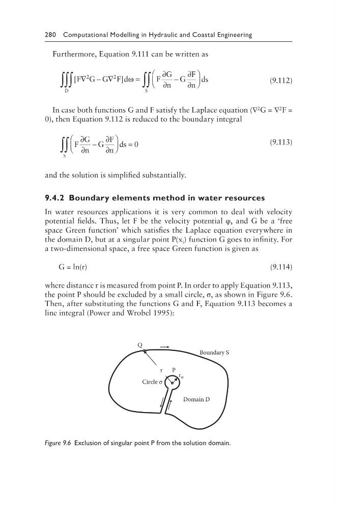
where distance r is measured from point P. In order to apply Equation 9.113,
the point P should be excluded by a small circle, σ, as shown in Figure 9.6.
Then, after substituting the functions G and F, Equation 9.113 becomes a
line integral (Power and Wrobel 1995):
Circle σ
Q
P
Boundary S
r o
Domain D
r
Figure 9.6 Exclusion of singular point P from the solution domain.
Furthermore, Equation 9.111 can be written as
[
]
F G G F d
F
G
n
G
F
n
ds
D
S
∇ − ∇
=
∂
∂
−
∂
∂
∫∫∫
∫∫
2
2
ω
(9.112)
In case both functions G and F satisfy the Laplace equation (∇ 2 G = ∇ 2 F =
0), then Equation 9.112 is reduced to the boundary integral
F
G
n
G
F
n
ds
S
∂
∂
−
∂
∂
=
∫∫
0
(9.113)
and the solution is simplified substantially.
9.4.2 Boundary elements method in water resources
In water resources applications it is very common to deal with velocity
potential fields. Thus, let F be the velocity potential φ, and G be a ‘free
space Green function’ which satisfies the Laplace equation everywhere in
the domain D, but at a singular point P(x i ) function G goes to infinity. For
a two-dimensional space, a free space Green function is given as
G = ln(r)
(9.114)
where distance r is measured from point P. In order to apply Equation 9.113,
the point P should be excluded by a small circle, σ, as shown in Figure 9.6.
Then, after substituting the functions G and F, Equation 9.113 becomes a
line integral (Power and Wrobel 1995):
Circle σ
Q
P
Boundary S
r o
Domain D
r
Figure 9.6 Exclusion of singular point P from the solution domain.