

Other numerical methods 283
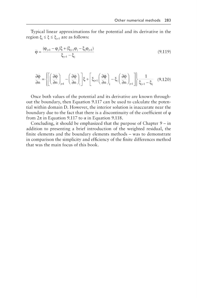
Typical linear approximations for the potential and its derivative in the
region ξ j ≤ ξ ≤ ξ j+1 are as follows:
ϕ
ϕ
ϕ ξ ξ ϕ ξϕ
ξ
ξ
=
−
+
−
−
+
+
+
+
(
) (
)
j
j
j
j j
j
j
1
1
1
1
j
(9.119)
∂
∂
=
∂
∂
−
∂
∂
+
∂
+
+
ϕ
ϕ
ϕ
ξ ξ
n
n
n
j
j
j
1
1
ϕ ϕ
ξ
ϕ
ξ
∂
−
∂
∂
+
n
n
j
j
j
j
1
1
+ + −
1
ξ j
(9.120)
Once both values of the potential and its derivative are known throughout the boundary, then Equation 9.117 can be used to calculate the potential within domain D. However, the interior solution is inaccurate near the
boundary due to the fact that there is a discontinuity of the coefficient of φ
from 2π in Equation 9.117 to α in Equation 9.118.
Concluding, it should be emphasized that the purpose of Chapter 9 – in
addition to presenting a brief introduction of the weighted residual, the
finite elements and the boundary elements methods – was to demonstrate
in comparison the simplicity and efficiency of the finite differences method
that was the main focus of this book.
Typical linear approximations for the potential and its derivative in the
region ξ j ≤ ξ ≤ ξ j+1 are as follows:
ϕ
ϕ
ϕ ξ ξ ϕ ξϕ
ξ
ξ
=
−
+
−
−
+
+
+
+
(
) (
)
j
j
j
j j
j
j
1
1
1
1
j
(9.119)
∂
∂
=
∂
∂
−
∂
∂
+
∂
+
+
ϕ
ϕ
ϕ
ξ ξ
n
n
n
j
j
j
1
1
ϕ ϕ
ξ
ϕ
ξ
∂
−
∂
∂
+
n
n
j
j
j
j
1
1
+ + −
1
ξ j
(9.120)
Once both values of the potential and its derivative are known throughout the boundary, then Equation 9.117 can be used to calculate the potential within domain D. However, the interior solution is inaccurate near the
boundary due to the fact that there is a discontinuity of the coefficient of φ
from 2π in Equation 9.117 to α in Equation 9.118.
Concluding, it should be emphasized that the purpose of Chapter 9 – in
addition to presenting a brief introduction of the weighted residual, the
finite elements and the boundary elements methods – was to demonstrate
in comparison the simplicity and efficiency of the finite differences method
that was the main focus of this book.