Other numerical methods 273
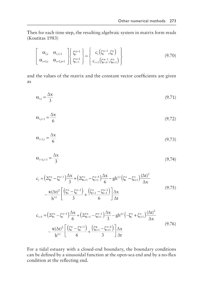
Then for each time step, the resulting algebraic system in matrix form reads
(Koutitas 1983)
α
α
α
α
ζ
ζ
i i
i i
i i
i i
i
n
i
n
,
,
,
,
+
+
+ +
+
+
+











1
1
1 1
1
1
1
  



 
=
(
)
(
)






−
+
+
−
+
c
c
i
i
n
i
n
i
i
n
i
n
ζ ζ
ζ ζ
1
1
1
1
1
,
,
 



(9.70)
and the values of the matrix and the constant vector coefficients are given
as
α i i
x
, =
∆
3
(9.71)
α i i
x
, + =
1
6
∆
(9.72)
α i i
x
+
=
1
6
,
∆
(9.73)
α i i
x
+ + =
1 1
3
,
∆
(9.74)
c
x
x gh
i
i
n
i
n
i
n
i
n
e
i
n
=
−
(
) +
−
(
) −
−
+
+
−
2
3
2
6
1
1
1
1
ζ ζ
ζ
ζ
ζ
∆
∆
( )
− −
(
)
−
−
(
) +
−
+
−
+
ζ
κ
ζ ζ
ζ
ζ
i
n
e
i
n
i
n
i
n
t
x
t
h
1
2
2
1
1
3
( )
( )
( )
∆
∆
∆
i i
n
x
t
+
−
(
)






1
1
6
∆
∆
(9.75)
c
x
x gh
i
i
n
i
n
i
n
i
n
e
+
−
+
+
−
=
−
(
) +
−
(
) −
−
1
1
1
1
1
2
6
2
3
ζ ζ
ζ
ζ
∆
∆
( )
ζ ζ ζ
κ
ζ ζ
ζ
i
n
i
n
e
i
n
i
n
i
t
x
t
h
+
(
)
−
−
(
) +
+
−
+
1
2
2
1
1
6
( )
( )
( )
∆
∆
∆
n n
i
n
x
t
−
(
)






+
−
ζ 1
1
3
∆
∆
(9.76)
For a tidal estuary with a closed-end boundary, the boundary conditions
can be defined by a sinusoidal function at the open-sea end and by a no-flux
condition at the reflecting end.