

272 Computational Modelling in Hydraulic and Coastal Engineering
equation) and for a hyperbolic system of differential equations (SaintVenant equations). In both cases, the resulting discretized algebraic equations are provided.
9.3.3.1 Telegrapher’s equation
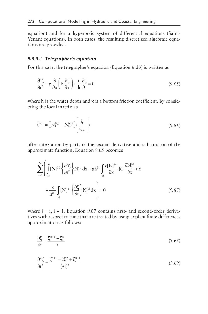
For this case, the telegrapher’s equation (Equation 6.23) is written as
∂
∂
−
∂
∂
∂
∂
+
∂
∂
=
2
2
0
ζ
ζ
κ ζ
t
g x
h x
h t
(9.65)
where h is the water depth and κ is a bottom friction coefficient. By considering the local matrix as
ζ
ζ
ζ
( )
( )
( )
e
i
e
i
e
i
i
i
i
i
N
N
=
+
+
1
1
(9.66)
after integration by parts of the second derivative and substitution of the
approximate function, Equation 9.65 becomes
[ ]
[ ] { }
( )
( )
( )
( )
(
N
t
N dx gh
N
x
N
e
j
e
e
e
j
∂
∂
+
∂
∂
∂
2
2
ζ
ζ
e e
e
e
e
x
dx
h
N
t
N
)
( )
( )
( )
( )
[ ]
∂
+
∂
∂
∫
∫
∑
=
e
e
M
1
κ
ζ
j j
e
e
dx
( )
( )
∫
= 0
(9.67)
where j = i, i + 1. Equation 9.67 contains first- and second-order derivatives with respect to time that are treated by using explicit finite differences
approximation as follows:
∂
∂
=
−
+
ζ ζ
ζ
t
t
i
n
i
n
1
(9.68)
∂
∂
=
−
+
+
−
2
2
1
1
2
2
ζ ζ
ζ ζ
t
t
i
n
i
n
i
n
( )
∆
(9.69)
equation) and for a hyperbolic system of differential equations (SaintVenant equations). In both cases, the resulting discretized algebraic equations are provided.
9.3.3.1 Telegrapher’s equation
For this case, the telegrapher’s equation (Equation 6.23) is written as
∂
∂
−
∂
∂
∂
∂
+
∂
∂
=
2
2
0
ζ
ζ
κ ζ
t
g x
h x
h t
(9.65)
where h is the water depth and κ is a bottom friction coefficient. By considering the local matrix as
ζ
ζ
ζ
( )
( )
( )
e
i
e
i
e
i
i
i
i
i
N
N
=
+
+
1
1
(9.66)
after integration by parts of the second derivative and substitution of the
approximate function, Equation 9.65 becomes
[ ]
[ ] { }
( )
( )
( )
( )
(
N
t
N dx gh
N
x
N
e
j
e
e
e
j
∂
∂
+
∂
∂
∂
2
2
ζ
ζ
e e
e
e
e
x
dx
h
N
t
N
)
( )
( )
( )
( )
[ ]
∂
+
∂
∂
∫
∫
∑
=
e
e
M
1
κ
ζ
j j
e
e
dx
( )
( )
∫
= 0
(9.67)
where j = i, i + 1. Equation 9.67 contains first- and second-order derivatives with respect to time that are treated by using explicit finite differences
approximation as follows:
∂
∂
=
−
+
ζ ζ
ζ
t
t
i
n
i
n
1
(9.68)
∂
∂
=
−
+
+
−
2
2
1
1
2
2
ζ ζ
ζ ζ
t
t
i
n
i
n
i
n
( )
∆
(9.69)