Other numerical methods 269
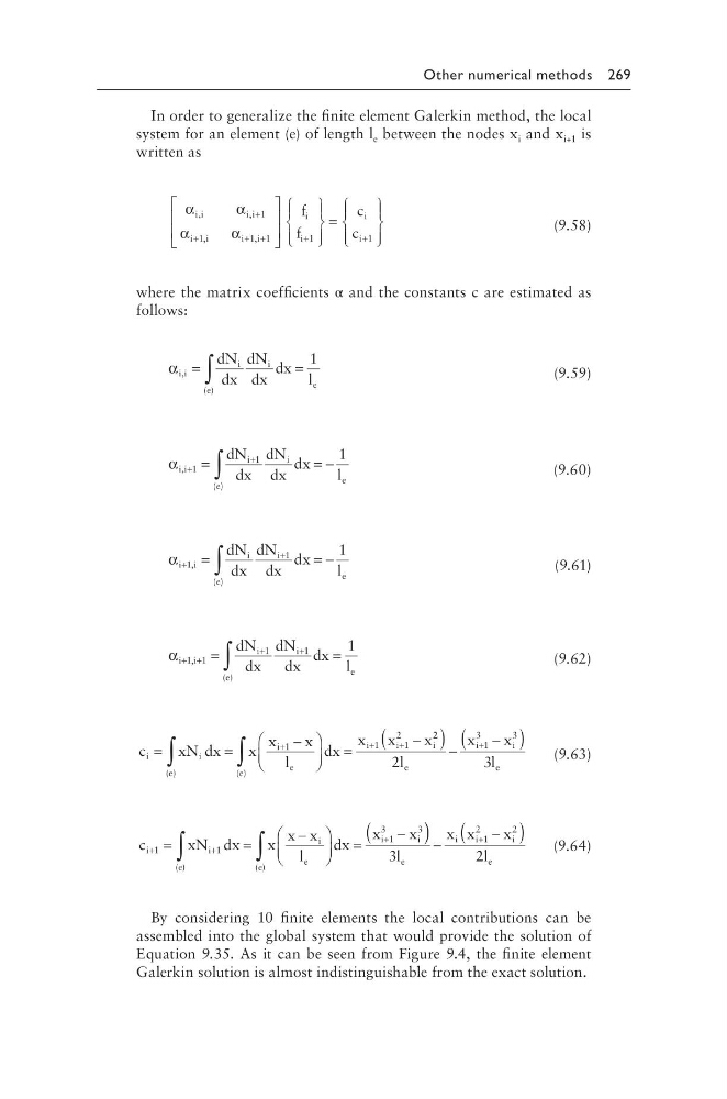
In order to generalize the finite element Galerkin method, the local
system for an element (e) of length l e between the nodes x i and x i+1 is
written as
α
α
α
α
i i
i i
i i
i i
i
i
f
f
,
,
,
,
+
+
+ +
+











 




1
1
1 1
1  
=



 



 
+
c
c
i
i 1
(9.58)
where the matrix coefficients α and the constants c are estimated as
follows:
α i i
i
i
e
e
dN
dx
dN
dx
dx l
,
( )
=
=
∫
1
(9.59)
α i i
i
i
e
e
dN
dx
dN
dx
dx
l
,
( )
+
+
=
= −
∫
1
1
1
(9.60)
α i i
i
i
e
e
dN
dx
dN
dx
dx
l
+
+
=
= −
∫
1
1
1
,
( )
(9.61)
α i i
i
i
e
e
dN
dx
dN
dx
dx l
+ +
+
+
=
=
∫
1 1
1
1
1
,
( )
(9.62)
c
xN dx
x
x
x
l
dx
x x
x
i
i
e
i
e
e
i
i
i
=
=
−

 

 
=
−
∫
∫
+
+
+
( )
( )
1
1
1
2
2 2
1
3
3
2
3
(
) −
−
(
)
+
l
x
x
l
e
i
i
e
(9.63)
c
x N dx
x
x x
l
dx
x
x
i
i
e
i
e
e
i
i
+
+
+
=
=
−

 

 
=
−
(
∫
∫
1
1
1
3
3
( )
( )
) ) −
−
(
)
+
3
2
1
2
2
l
x x
x
l
e
i
i
i
e
(9.64)
By considering 10 finite elements the local contributions can be
assembled into the global system that would provide the solution of
Equation 9.35. As it can be seen from Figure 9.4, the finite element
Galerkin solution is almost indistinguishable from the exact solution.