

268 Computational Modelling in Hydraulic and Coastal Engineering
Then for the functional to become stationary
dI f
df
f
f
[ ]
.
.
2
2
2
2
4
025 0
0625
=
−
= ⇒ =
(9.54)
Therefore, the value of the function at x = 0.5 (node 2) is equal to
0.625, and that coincides with the exact solution (Equation 9.40).
Galerkin method: Now the solution is being sought by using the
Galerkin method. For that purpose, Euler’s equation (Equation 9.35)
is used and again the solution domain is divided into two equal-length
finite elements. However, since the shape function is linear and Euler’s
equation is of the second-order, the second derivative of the trial function becomes zero. To avoid this difficulty, the theorem of integration
by parts is applied (Chung 1978):
du
dx
vdx uv
u
dv
dx
dx
x
x
x
x
x
x
=
−
∫
∫
1
2
1
2
1
2
(9.55)
where
u
df
dx
v N
=
=
,
(9.56)
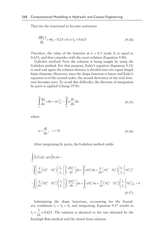
After integrating by parts, the Galerkin method yields
L f x
g x N dx
d
dx
N
N
f
f
[ ( )] ( )
( )
( )
−
{
} =
−
∫
0
1
2
1
1
2
1
1
2
+
∫
dN
dx
dx
xN dx
2
1
0
0 5
2
1
( )
.
( )
0 0
0 5
1
1
2
1
1
2
2
1
0
0 5
.
( )
( )
( ) .
∫
+
d
dx
N
N
f
f
N
− −
d
dx
N
N
f
f
dN
2
2
3
2
2
3
2
2
( )
( )
( )
d dx
dx
xN dx
d
dx
N
N
+
+
∫
∫
0 5
1
2
2
0 5
1
2
2
3
2
.
( )
.
( )
( )
=
f
f
N
2
3
2
1
0 5
1
0
( )
.
(9.57)
Substituting the shape functions, accounting for the boundary conditions f 1 = f 3 = 0, and integrating, Equation 9.57 results in
f 2
1
16
0 625
=
= .
. The solution is identical to the one obtained by the
Rayleigh-Ritz method and the closed form solution.
Then for the functional to become stationary
dI f
df
f
f
[ ]
.
.
2
2
2
2
4
025 0
0625
=
−
= ⇒ =
(9.54)
Therefore, the value of the function at x = 0.5 (node 2) is equal to
0.625, and that coincides with the exact solution (Equation 9.40).
Galerkin method: Now the solution is being sought by using the
Galerkin method. For that purpose, Euler’s equation (Equation 9.35)
is used and again the solution domain is divided into two equal-length
finite elements. However, since the shape function is linear and Euler’s
equation is of the second-order, the second derivative of the trial function becomes zero. To avoid this difficulty, the theorem of integration
by parts is applied (Chung 1978):
du
dx
vdx uv
u
dv
dx
dx
x
x
x
x
x
x
=
−
∫
∫
1
2
1
2
1
2
(9.55)
where
u
df
dx
v N
=
=
,
(9.56)
After integrating by parts, the Galerkin method yields
L f x
g x N dx
d
dx
N
N
f
f
[ ( )] ( )
( )
( )
−
{
} =
−
∫
0
1
2
1
1
2
1
1
2
+
∫
dN
dx
dx
xN dx
2
1
0
0 5
2
1
( )
.
( )
0 0
0 5
1
1
2
1
1
2
2
1
0
0 5
.
( )
( )
( ) .
∫
+
d
dx
N
N
f
f
N
− −
d
dx
N
N
f
f
dN
2
2
3
2
2
3
2
2
( )
( )
( )
d dx
dx
xN dx
d
dx
N
N
+
+
∫
∫
0 5
1
2
2
0 5
1
2
2
3
2
.
( )
.
( )
( )
=
f
f
N
2
3
2
1
0 5
1
0
( )
.
(9.57)
Substituting the shape functions, accounting for the boundary conditions f 1 = f 3 = 0, and integrating, Equation 9.57 results in
f 2
1
16
0 625
=
= .
. The solution is identical to the one obtained by the
Rayleigh-Ritz method and the closed form solution.