

Other numerical methods 267
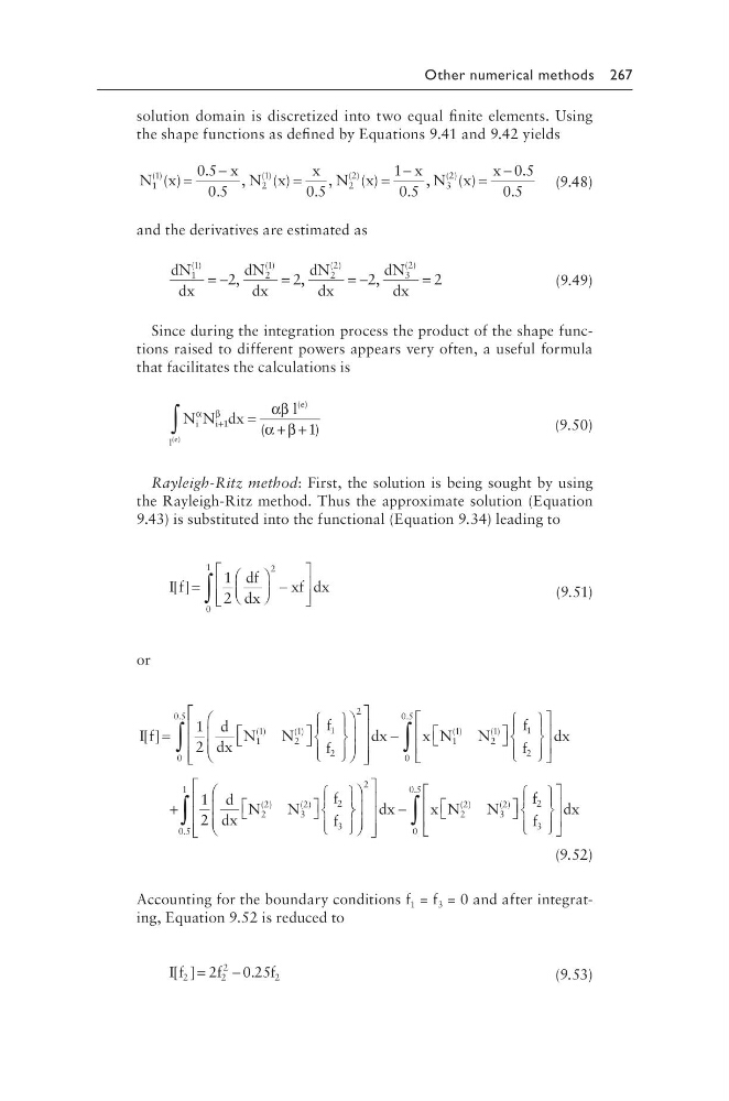
solution domain is discretized into two equal finite elements. Using
the shape functions as defined by Equations 9.41 and 9.42 yields
N x
x N x
x N x
x
1
1
2
1
2
2
0 5
0 5
0 5
1
0 5
( )
( )
( )
( )
.
.
,
( )
.
,
( )
.
=
−
=
=
− , ,
( )
.
.
( )
N x
x
3
2
0 5
0 5
=
−
(9.48)
and the derivatives are estimated as
dN
dx
dN
dx
dN
dx
dN
dx
1
1
2
1
2
2
3
2
2
2
2
2
( )
( )
( )
( )
,
,
,
= −
=
=−
=
(9.49)
Since during the integration process the product of the shape functions raised to different powers appears very often, a useful formula
that facilitates the calculations is
N N dx
l
i
i
l
e
e
α β
αβ
α β
+
∫
= + +
1
1
( )
( )
(
)
(9.50)
Rayleigh-Ritz method: First, the solution is being sought by using
the Rayleigh-Ritz method. Thus the approximate solution (Equation
9.43) is substituted into the functional (Equation 9.34) leading to
I f
df
dx
xf dx
[ ]=
−
∫
1
2
2
0
1
(9.51)
or
I f
d
dx
N
N
f
f
[ ]
( )
( )
=
1
2
1
1
2
1
1
2
2
−
∫
0
0 5
1
1
2
1
1
2
.
( )
( )
dx
x N
N
f
f
+
∫
0
0 5
2
2
3
2
2
3
1
2
.
( )
( )
dx
d
dx
N
N
f
f
−
∫
2
0 5
1
2
2
3
2
.
( )
( )
dx
x N
N
f f
f
dx
2
3
0
0 5
∫
.
(9.52)
Accounting for the boundary conditions f 1 = f 3 = 0 and after integrating, Equation 9.52 is reduced to
I f
f
f
[ ]
.
2
2
2
2
2
025
=
−
(9.53)
solution domain is discretized into two equal finite elements. Using
the shape functions as defined by Equations 9.41 and 9.42 yields
N x
x N x
x N x
x
1
1
2
1
2
2
0 5
0 5
0 5
1
0 5
( )
( )
( )
( )
.
.
,
( )
.
,
( )
.
=
−
=
=
− , ,
( )
.
.
( )
N x
x
3
2
0 5
0 5
=
−
(9.48)
and the derivatives are estimated as
dN
dx
dN
dx
dN
dx
dN
dx
1
1
2
1
2
2
3
2
2
2
2
2
( )
( )
( )
( )
,
,
,
= −
=
=−
=
(9.49)
Since during the integration process the product of the shape functions raised to different powers appears very often, a useful formula
that facilitates the calculations is
N N dx
l
i
i
l
e
e
α β
αβ
α β
+
∫
= + +
1
1
( )
( )
(
)
(9.50)
Rayleigh-Ritz method: First, the solution is being sought by using
the Rayleigh-Ritz method. Thus the approximate solution (Equation
9.43) is substituted into the functional (Equation 9.34) leading to
I f
df
dx
xf dx
[ ]=
−
∫
1
2
2
0
1
(9.51)
or
I f
d
dx
N
N
f
f
[ ]
( )
( )
=
1
2
1
1
2
1
1
2
2
−
∫
0
0 5
1
1
2
1
1
2
.
( )
( )
dx
x N
N
f
f
+
∫
0
0 5
2
2
3
2
2
3
1
2
.
( )
( )
dx
d
dx
N
N
f
f
−
∫
2
0 5
1
2
2
3
2
.
( )
( )
dx
x N
N
f f
f
dx
2
3
0
0 5
∫
.
(9.52)
Accounting for the boundary conditions f 1 = f 3 = 0 and after integrating, Equation 9.52 is reduced to
I f
f
f
[ ]
.
2
2
2
2
2
025
=
−
(9.53)