266 Computational Modelling in Hydraulic and Coastal Engineering
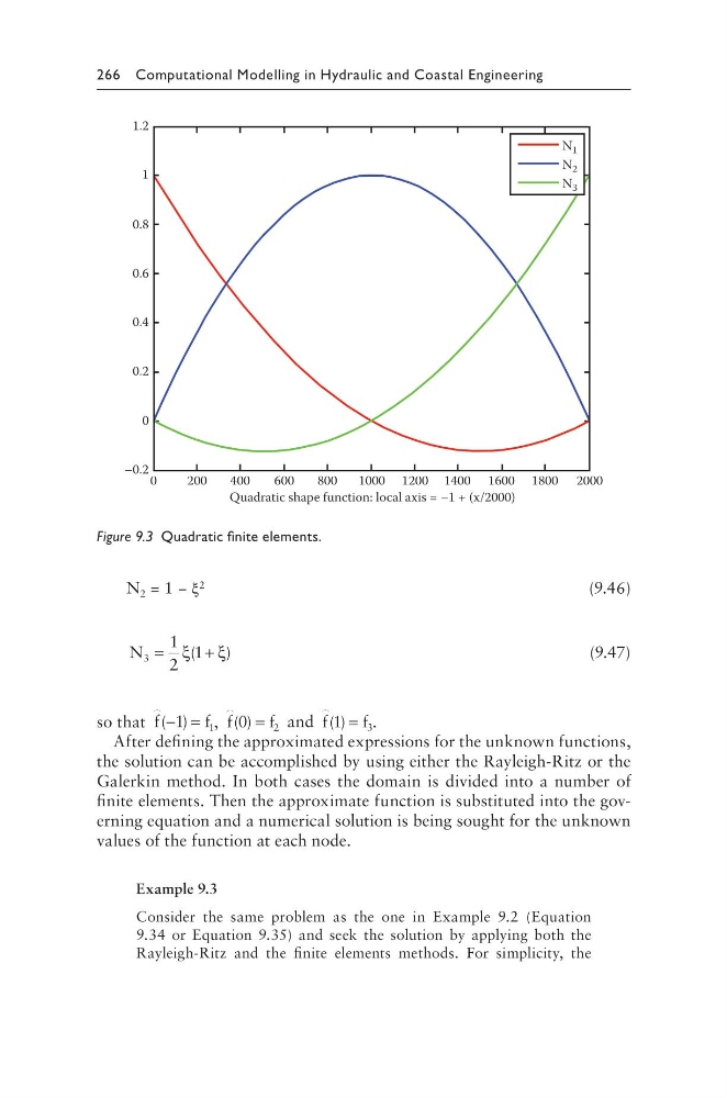
N 2 = 1 − ξ 2
(9.46)
N 3
1
2
1
=
+
ξ
ξ
(
)
(9.47)
so that

f
f
( )
− =
1 1 ,

f
f
( )
0
2
= and

f
f
( )
1
3
= .
After defining the approximated expressions for the unknown functions,
the solution can be accomplished by using either the Rayleigh-Ritz or the
Galerkin method. In both cases the domain is divided into a number of
finite elements. Then the approximate function is substituted into the governing equation and a numerical solution is being sought for the unknown
values of the function at each node.
Example 9.3
Consider the same problem as the one in Example 9.2 (Equation
9.34 or Equation 9.35) and seek the solution by applying both the
Rayleigh-Ritz and the finite elements methods. For simplicity, the
1.2
0.8
0.6
0.4
0.2
–0.2
0
1
0
200
400
600
800
1000 1200 1400 1600 1800 2000
Quadratic shape function: local axis = –1 + (x/2000)
N 1
N 2
N 3
Figure 9.3 Quadratic finite elements.