

Other numerical methods 265
N x
x x
x
x
x x
l
i
e
i
i
i
i
i
e
i
i
+
+
=
−
−
=
−
1
1
( )
( )
( )
(9.42)
where l i
e i
( )
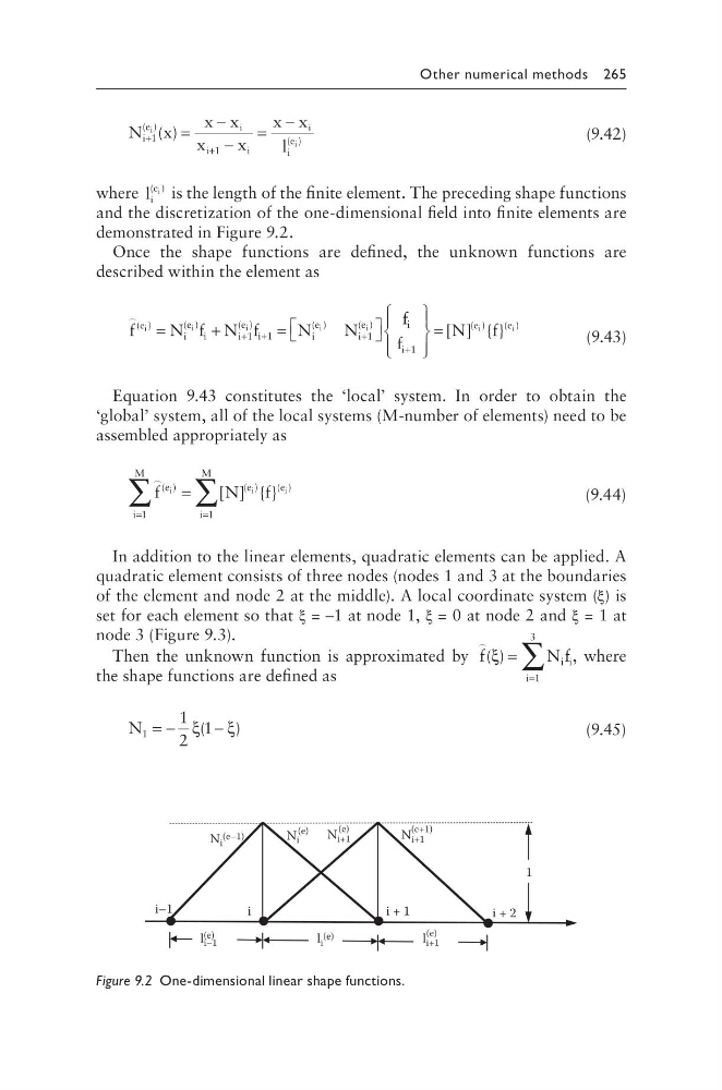
is the length of the finite element. The preceding shape functions
and the discretization of the one-dimensional field into finite elements are
demonstrated in Figure 9.2.
Once the shape functions are defined, the unknown functions are
described within the element as
f
N f N f
N
N
e
i
e
i
i
e
i
i
e
i
e
i
i
i
i
i
( )
( )
( )
( )
( )
=
+
=
+ +
+
1 1
1
f f
f
N
f
i
i
e
e
i
i
+
=
1
[ ] { }
( )
( )
(9.43)
Equation 9.43 constitutes the ‘local’ system. In order to obtain the
‘global’ system, all of the local systems (M-number of elements) need to be
assembled appropriately as
f
e
i
M
e
e
i
M
i
i
i
( )
( )
( )
[ ] { }
=
=
∑ ∑
=
1
1
N
f
(9.44)
In addition to the linear elements, quadratic elements can be applied. A
quadratic element consists of three nodes (nodes 1 and 3 at the boundaries
of the element and node 2 at the middle). A local coordinate system (ξ) is
set for each element so that ξ = –1 at node 1, ξ = 0 at node 2 and ξ = 1 at
node 3 (Figure 9.3).
Then the unknown function is approximated by
f
Nf i i
i
( )
ξ =
=
∑
1
3
, where
the shape functions are defined as
N 1
1
2
1
= −
−
ξ
ξ
(
)
(9.45)
N i
(e–1)
N i
N i+1
N i+1
i + 2
i + 1
i–1
i
1
l i–1
l i
(e)
l i+1
(e)
(e)
(e+1)
(e)
(e)
Figure 9.2 One-dimensional linear shape functions.
N x
x x
x
x
x x
l
i
e
i
i
i
i
i
e
i
i
+
+
=
−
−
=
−
1
1
( )
( )
( )
(9.42)
where l i
e i
( )
is the length of the finite element. The preceding shape functions
and the discretization of the one-dimensional field into finite elements are
demonstrated in Figure 9.2.
Once the shape functions are defined, the unknown functions are
described within the element as
f
N f N f
N
N
e
i
e
i
i
e
i
i
e
i
e
i
i
i
i
i
( )
( )
( )
( )
( )
=
+
=
+ +
+
1 1
1
f f
f
N
f
i
i
e
e
i
i
+
=
1
[ ] { }
( )
( )
(9.43)
Equation 9.43 constitutes the ‘local’ system. In order to obtain the
‘global’ system, all of the local systems (M-number of elements) need to be
assembled appropriately as
f
e
i
M
e
e
i
M
i
i
i
( )
( )
( )
[ ] { }
=
=
∑ ∑
=
1
1
N
f
(9.44)
In addition to the linear elements, quadratic elements can be applied. A
quadratic element consists of three nodes (nodes 1 and 3 at the boundaries
of the element and node 2 at the middle). A local coordinate system (ξ) is
set for each element so that ξ = –1 at node 1, ξ = 0 at node 2 and ξ = 1 at
node 3 (Figure 9.3).
Then the unknown function is approximated by
f
Nf i i
i
( )
ξ =
=
∑
1
3
, where
the shape functions are defined as
N 1
1
2
1
= −
−
ξ
ξ
(
)
(9.45)
N i
(e–1)
N i
N i+1
N i+1
i + 2
i + 1
i–1
i
1
l i–1
l i
(e)
l i+1
(e)
(e)
(e+1)
(e)
(e)
Figure 9.2 One-dimensional linear shape functions.