

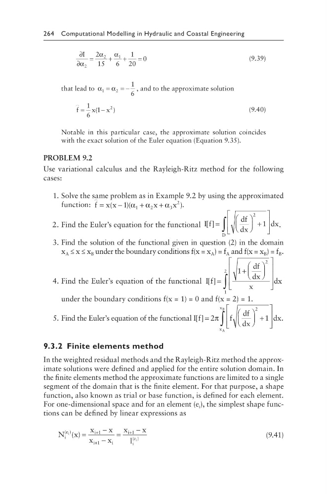
264 Computational Modelling in Hydraulic and Coastal Engineering
∂
∂
=
+
+
=
I
α
α
α
2
2
1
2
15
6
1
20
0
(9.39)
that lead to α α
1
2
1
6
=
=− , and to the approximate solution
f
x
x
=
−
1
6
1
2
(
)
(9.40)
Notable in this particular case, the approximate solution coincides
with the exact solution of the Euler equation (Equation 9.35).
PROBLEM 9.2
Use variational calculus and the Rayleigh-Ritz method for the following
cases:
1. Solve the same problem as in Example 9.2 by using the approximated
function:
f x x
x
x
=
−
+
+
(
)(
)
1 1
2
3
2
α α
α
.
2. Find the Euler’s equation for the functional I f
df
dx
dx
D
[ ] =
+
∫
2
1
.
3. Find the solution of the functional given in question (2) in the domain
x A ≤ x ≤ x B under the boundary conditions f(x = x A ) = f A and f(x = x B ) = f B .
4. Find the Euler’s equation of the functional I f
df
dx
x
dx
[ ] =
+
∫
1
2
1
2
under the boundary conditions f(x = 1) = 0 and f(x = 2) = 1.
5. Find the Euler’s equation of the functional I f
f
df
dx
dx
x
x
A
B
[ ] =
+
∫
2
1
2
π
.
9.3.2 Finite elements method
In the weighted residual methods and the Rayleigh-Ritz method the approximate solutions were defined and applied for the entire solution domain. In
the finite elements method the approximate functions are limited to a single
segment of the domain that is the finite element. For that purpose, a shape
function, also known as trial or base function, is defined for each element.
For one-dimensional space and for an element (e i ), the simplest shape functions can be defined by linear expressions as
N x
x
x
x
x
x
x
l
i
e
i
i
i
i
i
e
i
i
( )
( )
( ) =
−
−
=
−
+
+
+
1
1
1
(9.41)
∂
∂
=
+
+
=
I
α
α
α
2
2
1
2
15
6
1
20
0
(9.39)
that lead to α α
1
2
1
6
=
=− , and to the approximate solution
f
x
x
=
−
1
6
1
2
(
)
(9.40)
Notable in this particular case, the approximate solution coincides
with the exact solution of the Euler equation (Equation 9.35).
PROBLEM 9.2
Use variational calculus and the Rayleigh-Ritz method for the following
cases:
1. Solve the same problem as in Example 9.2 by using the approximated
function:
f x x
x
x
=
−
+
+
(
)(
)
1 1
2
3
2
α α
α
.
2. Find the Euler’s equation for the functional I f
df
dx
dx
D
[ ] =
+
∫
2
1
.
3. Find the solution of the functional given in question (2) in the domain
x A ≤ x ≤ x B under the boundary conditions f(x = x A ) = f A and f(x = x B ) = f B .
4. Find the Euler’s equation of the functional I f
df
dx
x
dx
[ ] =
+
∫
1
2
1
2
under the boundary conditions f(x = 1) = 0 and f(x = 2) = 1.
5. Find the Euler’s equation of the functional I f
f
df
dx
dx
x
x
A
B
[ ] =
+
∫
2
1
2
π
.
9.3.2 Finite elements method
In the weighted residual methods and the Rayleigh-Ritz method the approximate solutions were defined and applied for the entire solution domain. In
the finite elements method the approximate functions are limited to a single
segment of the domain that is the finite element. For that purpose, a shape
function, also known as trial or base function, is defined for each element.
For one-dimensional space and for an element (e i ), the simplest shape functions can be defined by linear expressions as
N x
x
x
x
x
x
x
l
i
e
i
i
i
i
i
e
i
i
( )
( )
( ) =
−
−
=
−
+
+
+
1
1
1
(9.41)