

270 Computational Modelling in Hydraulic and Coastal Engineering
Computer code 9.1
% Example 9.1 Finite Element Method
% dx = Length of the finite element;
% imax = Number of nodes;
% a = Matrix coefficients;
% c = Vector of constants;
% f = value of functions at the nodes;
dx = 0.1;
imax = 11;
imax1 = imax-1;
for i = 1:imax
f(i) = 0;
c(i) = 0;
for j = 1:imax
a(i,j) = 0;
end
end
for i = 1:imax1
a(i,i) = a(i,i)+1/dx;
a(i,i+1) = a(i,i+1)-1/dx;
a(i+1,i) = a(i+1,i)-1/dx;
a(i+1,i+1) = a(i+1,i+1)+1/dx;
c(i) = c(i)+dx^2*(i*(i^2-(i-1)^2)/2-(i^3-(i-1)^3)/3);
c(i+1) = c(i+1)+dx^2*((i^3-(i-1)^3)/3-(i-1)*(i^2-(i-1)^2)/2);
0.07
0.06
0.05
0.04
0.03
0.02
0.01
0 0
1
2
3
4
5
6
7
8
9
10
Solution domain × 10 –1
Function f(x)
FE Galerkin
Exact solution
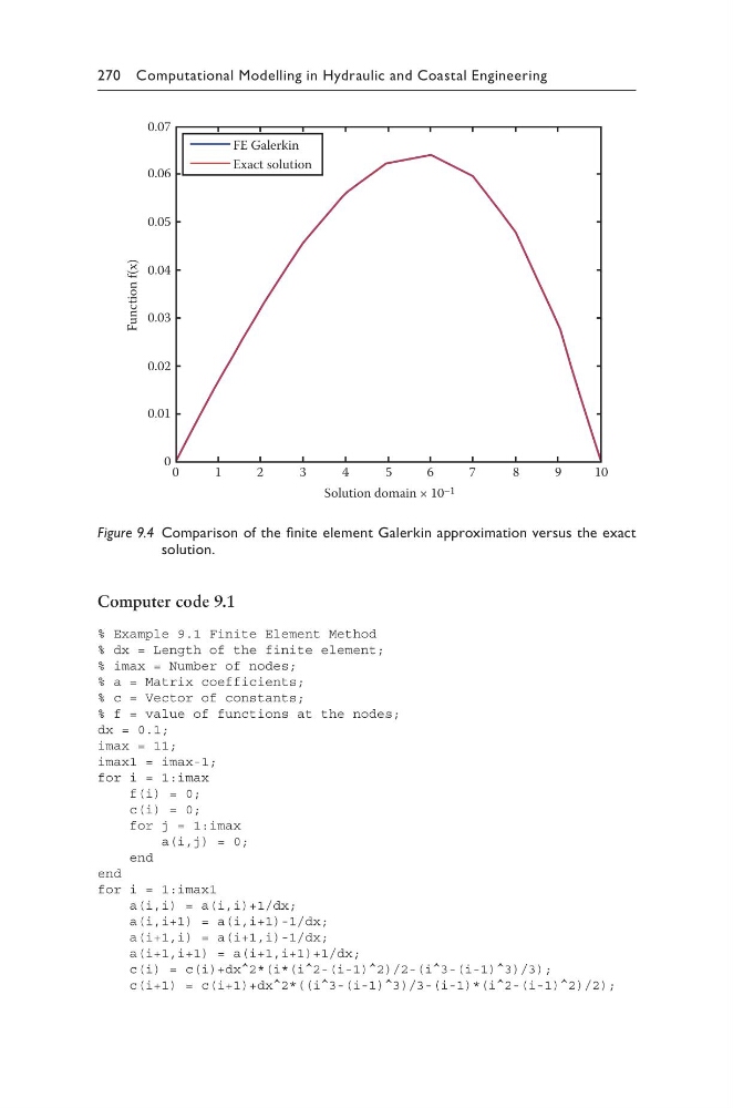
Figure 9.4 Comparison of the finite element Galerkin approximation versus the exact
solution.
Computer code 9.1
% Example 9.1 Finite Element Method
% dx = Length of the finite element;
% imax = Number of nodes;
% a = Matrix coefficients;
% c = Vector of constants;
% f = value of functions at the nodes;
dx = 0.1;
imax = 11;
imax1 = imax-1;
for i = 1:imax
f(i) = 0;
c(i) = 0;
for j = 1:imax
a(i,j) = 0;
end
end
for i = 1:imax1
a(i,i) = a(i,i)+1/dx;
a(i,i+1) = a(i,i+1)-1/dx;
a(i+1,i) = a(i+1,i)-1/dx;
a(i+1,i+1) = a(i+1,i+1)+1/dx;
c(i) = c(i)+dx^2*(i*(i^2-(i-1)^2)/2-(i^3-(i-1)^3)/3);
c(i+1) = c(i+1)+dx^2*((i^3-(i-1)^3)/3-(i-1)*(i^2-(i-1)^2)/2);
0.07
0.06
0.05
0.04
0.03
0.02
0.01
0 0
1
2
3
4
5
6
7
8
9
10
Solution domain × 10 –1
Function f(x)
FE Galerkin
Exact solution
Figure 9.4 Comparison of the finite element Galerkin approximation versus the exact
solution.