Flow in porous media 183
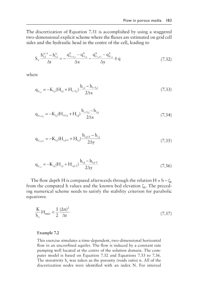
The discretization of Equation 7.31 is accomplished by using a staggered
two-dimensional explicit scheme where the fluxes are estimated on grid cell
sides and the hydraulic head in the centre of the cell, leading to
S
h
h
t
q
q
x
q
q
x
i j
n
i j
n
x
n
x
n
y
n
i j
i j
i j
,
,
,
,
,
+
−
= −
−
−
−
+
+
1
1
1
∆
∆
y y
n
i j
y
q
,
∆
±
(7.32)
where
q
K H
H
h
h
x
x
i j
ij
i j
i j
i j
i j
,
,
,
,
,
,
(
)
= −
+
−
−
−
1
1
2∆
(7.33)
q
K H
H
h
h
x
x
i j
i j
ij
i j
i j
i j
+
= −
+
−
+
+
1
1
1
2
,
,
,
,
,
,
(
)
∆
(7.34)
q
K H
H
h
h
y
y
i j
ij
i j
i j
i j
i j
,
,
,
,
,
,
(
)
+
= −
+
−
+
+
1
1
1
2∆
(7.35)
q
K H
H
h
h
y
y
i j
ij
ij
i j
i j
i j
,
,
,
,
,
,
(
)
= −
+
−
−
−
1
1
2∆
(7.36)
The flow depth H is computed afterwards through the relation H = h – ζ b
from the computed h values and the known bed elevation ζ b . The preceding numerical scheme needs to satisfy the stability criterion for parabolic
equations:
K
S
H
x
t
x
max
( )
<
1
2
2
∆
∆
(7.37)
Example 7.2
This exercise simulates a time-dependent, two-dimensional horizontal
flow in an unconfined aquifer. The flow is induced by a constant rate
pumping well located at the centre of the solution domain. The computer model is based on Equation 7.32 and Equations 7.33 to 7.36.
The storativity S x was taken as the porosity (voids ratio) n. All of the
discretization nodes were identified with an index N. For internal