

182 Computational Modelling in Hydraulic and Coastal Engineering
7.2.2 Horizontal two-dimensional groundwater flows
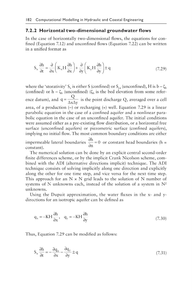
In the case of horizontally two-dimensional flows, the equations for confined (Equation 7.12) and unconfined flows (Equation 7.22) can be written
in a unified format as
S
h
t
x
K H
h
x
y
K H
h
y
q
x
x
y
∂
∂
=
∂
∂
∂
∂
+
∂
∂
∂
∂
±
(7.29)
where the ‘storativity’ S x is either S (confined) or S ya (unconfined), H is b – ζ b
(confined) or h – ζ b (unconfined) (ζ b is the bed elevation from some reference datum), and q
Q
x y
= ∆ ∆
is the point discharge Q, averaged over a cell
area, of a production (–) or recharging (+) well. Equation 7.29 is a linear
parabolic equation in the case of a confined aquifer and a nonlinear parabolic equation in the case of an unconfined aquifer. The initial conditions
were assumed either as a pre-existing flow distribution, or a horizontal free
surface (unconfined aquifers) or piezometric surface (confined aquifers),
implying no initial flow. The most common boundary conditions are either
impermeable lateral boundaries
∂
∂
=
h
n
0 or constant head boundaries (h =
constant).
The numerical solution can be done by an explicit central second-order
finite differences scheme, or by the implicit Crank Nicolson scheme, combined with the ADI (alternative directions implicit) technique. The ADI
technique consists of solving implicitly along one direction and explicitly
along the other for one time step, and vice versa for the next time step.
This approach for an N × N grid leads to the solution of N number of
systems of N unknowns each, instead of the solution of a system in N 2
unknowns.
Using the Dupuit approximation, the water fluxes in the x- and ydirections for an isotropic aquifer can be defined as
q
KH
h
x
q
KH
h
y
x
y
= −
∂
∂
= −
∂
∂
,
(7.30)
Thus, Equation 7.29 can be modified as follows:
S
h
t
q
x
q
y
q
x
x
y
∂
∂
= −
∂
∂
−
∂
∂
±
(7.31)
7.2.2 Horizontal two-dimensional groundwater flows
In the case of horizontally two-dimensional flows, the equations for confined (Equation 7.12) and unconfined flows (Equation 7.22) can be written
in a unified format as
S
h
t
x
K H
h
x
y
K H
h
y
q
x
x
y
∂
∂
=
∂
∂
∂
∂
+
∂
∂
∂
∂
±
(7.29)
where the ‘storativity’ S x is either S (confined) or S ya (unconfined), H is b – ζ b
(confined) or h – ζ b (unconfined) (ζ b is the bed elevation from some reference datum), and q
Q
x y
= ∆ ∆
is the point discharge Q, averaged over a cell
area, of a production (–) or recharging (+) well. Equation 7.29 is a linear
parabolic equation in the case of a confined aquifer and a nonlinear parabolic equation in the case of an unconfined aquifer. The initial conditions
were assumed either as a pre-existing flow distribution, or a horizontal free
surface (unconfined aquifers) or piezometric surface (confined aquifers),
implying no initial flow. The most common boundary conditions are either
impermeable lateral boundaries
∂
∂
=
h
n
0 or constant head boundaries (h =
constant).
The numerical solution can be done by an explicit central second-order
finite differences scheme, or by the implicit Crank Nicolson scheme, combined with the ADI (alternative directions implicit) technique. The ADI
technique consists of solving implicitly along one direction and explicitly
along the other for one time step, and vice versa for the next time step.
This approach for an N × N grid leads to the solution of N number of
systems of N unknowns each, instead of the solution of a system in N 2
unknowns.
Using the Dupuit approximation, the water fluxes in the x- and ydirections for an isotropic aquifer can be defined as
q
KH
h
x
q
KH
h
y
x
y
= −
∂
∂
= −
∂
∂
,
(7.30)
Thus, Equation 7.29 can be modified as follows:
S
h
t
q
x
q
y
q
x
x
y
∂
∂
= −
∂
∂
−
∂
∂
±
(7.31)