Flow in porous media 181
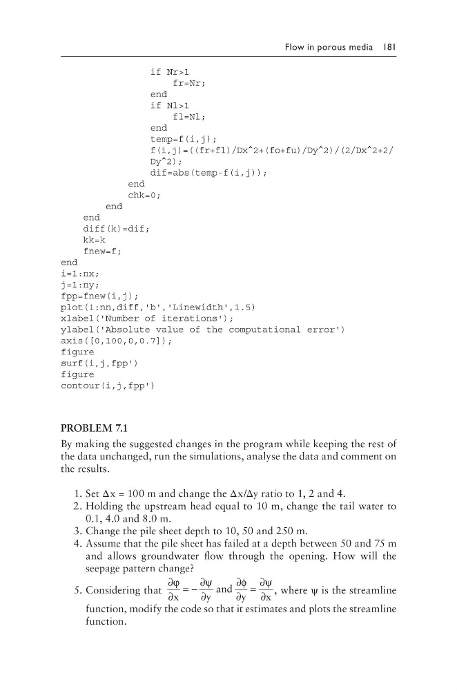
if Nr>1
fr=Nr;
end
if Nl>1
fl=Nl;
end
temp=f(i,j);
f(i,j)=((fr+fl)/Dx^2+(fo+fu)/Dy^2)/(2/Dx^2+2/
Dy^2);
dif=abs(temp-f(i,j));
end
chk=0;
end
end
diff(k)=dif;
kk=k
fnew=f;
end
i=1:nx;
j=1:ny;
fpp=fnew(i,j);
plot(1:nn,diff,'b','Linewidth',1.5)
xlabel('Number of iterations');
ylabel('Absolute value of the computational error')
axis([0,100,0,0.7]);
figure
surf(i,j,fpp')
figure
contour(i,j,fpp')
PROBLEM 7.1
By making the suggested changes in the program while keeping the rest of
the data unchanged, run the simulations, analyse the data and comment on
the results.
1. Set Δx = 100 m and change the Δx/Δy ratio to 1, 2 and 4.
2. Holding the upstream head equal to 10 m, change the tail water to
0.1, 4.0 and 8.0 m.
3. Change the pile sheet depth to 10, 50 and 250 m.
4. Assume that the pile sheet has failed at a depth between 50 and 75 m
and allows groundwater flow through the opening. How will the
seepage pattern change?
5. Considering that
∂
∂
= −
∂
∂
∂
∂
=
∂
∂
ϕ
ψ
φ
ψ
x
y
and y
x
, where ψ is the streamline
function, modify the code so that it estimates and plots the streamline
function.