

174 Computational Modelling in Hydraulic and Coastal Engineering
∂
∂
∂
∂
=
∂
∂
+
∂
∂
≈
∂
∂
≈
∂
y
h
h
y
h
y
h
h
y
h
h
y
h o
2
2
2
2
2
2
h h
y
∂
2
(7.25)
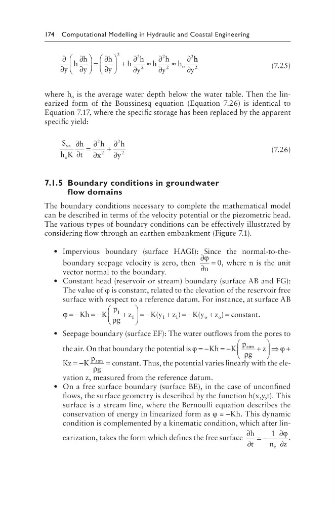
where h o is the average water depth below the water table. Then the linearized form of the Boussinesq equation (Equation 7.26) is identical to
Equation 7.17, where the specific storage has been replaced by the apparent
specific yield:
S
h K
h
t
h
x
h
y
ya
o
∂
∂
=
∂
∂
+
∂
∂
2
2
2
2
(7.26)
7.1.5 Boundary conditions in groundwater
flow domains
The boundary conditions necessary to complete the mathematical model
can be described in terms of the velocity potential or the piezometric head.
The various types of boundary conditions can be effectively illustrated by
considering flow through an earthen embankment (Figure 7.1).
• Impervious boundary (surface HAGI): Since the normal-to-theboundary seepage velocity is zero, then
∂
∂
=
ϕ
n
0, where n is the unit
vector normal to the boundary.
• Constant head (reservoir or stream) boundary (surface AB and FG):
The value of φ is constant, related to the elevation of the reservoir free
surface with respect to a reference datum. For instance, at surface AB
ϕ
ρ
= −
= −
+
= −
+ =−
+
=
Kh
K
p
g
z
Ky z
K y z
o
o
1
1
1
1
(
)
(
) consta ant.
• Seepage boundary (surface EF): The water outflows from the pores to
the air. On that boundary the potential is ϕ
ρ
ϕ
= −
= −
+
⇒ +
Kh
K
p
g
z
atm
Kz
K
p
g
atm
= −
=
ρ
constant. Thus, the potential varies linearly with the elevation z, measured from the reference datum.
• On a free surface boundary (surface BE), in the case of unconfined
flows, the surface geometry is described by the function h(x,y,t). This
surface is a stream line, where the Bernoulli equation describes the
conservation of energy in linearized form as φ = –Kh. This dynamic
condition is complemented by a kinematic condition, which after linearization, takes the form which defines the free surface
∂
∂
= −
∂
∂
h
t
n z
e
1 ϕ .
∂
∂
∂
∂
=
∂
∂
+
∂
∂
≈
∂
∂
≈
∂
y
h
h
y
h
y
h
h
y
h
h
y
h o
2
2
2
2
2
2
h h
y
∂
2
(7.25)
where h o is the average water depth below the water table. Then the linearized form of the Boussinesq equation (Equation 7.26) is identical to
Equation 7.17, where the specific storage has been replaced by the apparent
specific yield:
S
h K
h
t
h
x
h
y
ya
o
∂
∂
=
∂
∂
+
∂
∂
2
2
2
2
(7.26)
7.1.5 Boundary conditions in groundwater
flow domains
The boundary conditions necessary to complete the mathematical model
can be described in terms of the velocity potential or the piezometric head.
The various types of boundary conditions can be effectively illustrated by
considering flow through an earthen embankment (Figure 7.1).
• Impervious boundary (surface HAGI): Since the normal-to-theboundary seepage velocity is zero, then
∂
∂
=
ϕ
n
0, where n is the unit
vector normal to the boundary.
• Constant head (reservoir or stream) boundary (surface AB and FG):
The value of φ is constant, related to the elevation of the reservoir free
surface with respect to a reference datum. For instance, at surface AB
ϕ
ρ
= −
= −
+
= −
+ =−
+
=
Kh
K
p
g
z
Ky z
K y z
o
o
1
1
1
1
(
)
(
) consta ant.
• Seepage boundary (surface EF): The water outflows from the pores to
the air. On that boundary the potential is ϕ
ρ
ϕ
= −
= −
+
⇒ +
Kh
K
p
g
z
atm
Kz
K
p
g
atm
= −
=
ρ
constant. Thus, the potential varies linearly with the elevation z, measured from the reference datum.
• On a free surface boundary (surface BE), in the case of unconfined
flows, the surface geometry is described by the function h(x,y,t). This
surface is a stream line, where the Bernoulli equation describes the
conservation of energy in linearized form as φ = –Kh. This dynamic
condition is complemented by a kinematic condition, which after linearization, takes the form which defines the free surface
∂
∂
= −
∂
∂
h
t
n z
e
1 ϕ .