

Flow in porous media 173
of the water table. Therefore the specific storage S s = 0 and Equation 7.12
reduces to
∂
∂
∂
∂
+
∂
∂
∂
∂
+
∂
∂
∂
∂
x
K
h
x
y
K
h
y
z
K
h
z
x
y
z
= = 0
(7.19)
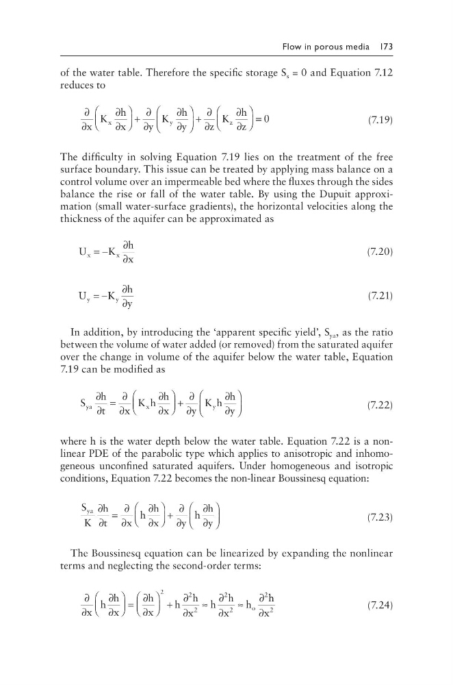
The difficulty in solving Equation 7.19 lies on the treatment of the free
surface boundary. This issue can be treated by applying mass balance on a
control volume over an impermeable bed where the fluxes through the sides
balance the rise or fall of the water table. By using the Dupuit approximation (small water-surface gradients), the horizontal velocities along the
thickness of the aquifer can be approximated as
U
K
h
x
x
x
= −
∂
∂
(7.20)
U
K
h
y
y
y
= −
∂
∂
(7.21)
In addition, by introducing the ‘apparent specific yield’, S ya , as the ratio
between the volume of water added (or removed) from the saturated aquifer
over the change in volume of the aquifer below the water table, Equation
7.19 can be modified as
S
h
t
x
K h
h
x
y
K h
h
y
ya
x
y
∂
∂
=
∂
∂
∂
∂
+
∂
∂
∂
∂
(7.22)
where h is the water depth below the water table. Equation 7.22 is a nonlinear PDE of the parabolic type which applies to anisotropic and inhomogeneous unconfined saturated aquifers. Under homogeneous and isotropic
conditions, Equation 7.22 becomes the non-linear Boussinesq equation:
S
K
h
t
x
h
h
x
y
h
h
y
ya ∂
∂
=
∂
∂
∂
∂
+
∂
∂
∂
∂
(7.23)
The Boussinesq equation can be linearized by expanding the nonlinear
terms and neglecting the second-order terms:
∂
∂
∂
∂
=
∂
∂
+
∂
∂
≈
∂
∂
≈
∂
x
h
h
x
h
x
h
h
x
h
h
x
h o
2
2
2
2
2
2
h h
x
∂
2
(7.24)
of the water table. Therefore the specific storage S s = 0 and Equation 7.12
reduces to
∂
∂
∂
∂
+
∂
∂
∂
∂
+
∂
∂
∂
∂
x
K
h
x
y
K
h
y
z
K
h
z
x
y
z
= = 0
(7.19)
The difficulty in solving Equation 7.19 lies on the treatment of the free
surface boundary. This issue can be treated by applying mass balance on a
control volume over an impermeable bed where the fluxes through the sides
balance the rise or fall of the water table. By using the Dupuit approximation (small water-surface gradients), the horizontal velocities along the
thickness of the aquifer can be approximated as
U
K
h
x
x
x
= −
∂
∂
(7.20)
U
K
h
y
y
y
= −
∂
∂
(7.21)
In addition, by introducing the ‘apparent specific yield’, S ya , as the ratio
between the volume of water added (or removed) from the saturated aquifer
over the change in volume of the aquifer below the water table, Equation
7.19 can be modified as
S
h
t
x
K h
h
x
y
K h
h
y
ya
x
y
∂
∂
=
∂
∂
∂
∂
+
∂
∂
∂
∂
(7.22)
where h is the water depth below the water table. Equation 7.22 is a nonlinear PDE of the parabolic type which applies to anisotropic and inhomogeneous unconfined saturated aquifers. Under homogeneous and isotropic
conditions, Equation 7.22 becomes the non-linear Boussinesq equation:
S
K
h
t
x
h
h
x
y
h
h
y
ya ∂
∂
=
∂
∂
∂
∂
+
∂
∂
∂
∂
(7.23)
The Boussinesq equation can be linearized by expanding the nonlinear
terms and neglecting the second-order terms:
∂
∂
∂
∂
=
∂
∂
+
∂
∂
≈
∂
∂
≈
∂
x
h
h
x
h
x
h
h
x
h
h
x
h o
2
2
2
2
2
2
h h
x
∂
2
(7.24)